Unlocking Drug Discovery: How to Apply the InVEST Habitat Quality Model for High-Value Target Screening
This article provides a comprehensive guide for biomedical researchers on adapting the InVEST Habitat Quality model—a conservation biology tool—for the computational screening of disease-relevant biological targets and pathways.
Unlocking Drug Discovery: How to Apply the InVEST Habitat Quality Model for High-Value Target Screening
Abstract
This article provides a comprehensive guide for biomedical researchers on adapting the InVEST Habitat Quality model—a conservation biology tool—for the computational screening of disease-relevant biological targets and pathways. We explore the foundational principles that enable this cross-disciplinary translation, detail a step-by-step methodological workflow from data preparation to analysis, address common troubleshooting and optimization challenges, and critically examine validation frameworks against established in silico screening methods. The aim is to empower scientists with a robust, ecosystem-inspired framework to prioritize high-value 'source' targets at the earliest stages of drug development, potentially increasing pipeline efficiency and success rates.
From Ecosystems to Drug Targets: The Foundational Logic of Repurposing InVEST HQ
Translating Ecological 'Habitat Quality' to Biological 'Target Value'
Within the context of screening for novel bioactive compounds (e.g., from microbial sources in diverse habitats), a conceptual bridge is needed between ecological integrity and therapeutic potential. In InVEST model terms, 'Habitat Quality' is a metric reflecting the ability of an ecosystem to support species, influenced by habitat extent and threat intensity. In drug discovery, the analogous 'Target Value' is a quantifiable measure of a biological target's therapeutic relevance and 'druggability'.
Translation Framework Table:
| Ecological Concept (InVEST) | Biological/Drug Discovery Analogue | Key Quantifiable Metrics |
|---|---|---|
| Habitat Extent & Type | Target Expression & Localization | Tissue-specific mRNA/protein levels (TPM, IHC scores); subcellular localization. |
| Threat Intensity & Proximity | Disease Linkage & Pathway Dysregulation | Genetic association scores (GWAS p-values); pathway enrichment FDR; mutational frequency in disease. |
| Habitat Sensitivity | Target Essentiality & Phenotypic Impact | CRISPR knockout viability scores (Chronos, DEMETER); RNAi phenotypic Z-scores. |
| Overall Habitat Quality Index | Integrated Target Value Score | Composite score weighting druggability, safety, disease linkage, and commercial viability. |
Application Notes: From Habitat to Hit
Prioritizing Sampling Sites Using Ecological Metrics
High InVEST Habitat Quality scores indicate biodiverse, stable ecosystems. Such sites are prioritized for microbial sampling.
Table: Correlation Metrics Between Ecological and Molecular Diversity
| Study Site (Hypothetical) | InVEST HQ Score | Soil Microbial Alpha Diversity (Shannon Index) | Unique Biosynthetic Gene Clusters (BGCs) per Gb Metagenome |
|---|---|---|---|
| Protected Old-Growth Forest | 0.92 | 9.8 ± 0.3 | 145 ± 12 |
| Managed Agricultural Land | 0.45 | 6.1 ± 0.5 | 62 ± 8 |
| Recovering Post-Industrial | 0.68 | 7.9 ± 0.4 | 98 ± 10 |
Defining Biological 'Target Value' for Screening
A high-value target is essential in the disease pathway, has a druggable pocket, and exhibits a safe modulation profile.
Table: Target Value Scoring Matrix (Example)
| Parameter | Weight | Sub-Score Metrics | High-Value Example (Score) |
|---|---|---|---|
| Genetic Validation | 30% | LoF/GoF phenotype concordance; GWAS significance. | PCSK9 (30/30) |
| Druggability | 25% | 3D structure known; small molecule precedent. | Kinase domain (25/25) |
| Safety | 20% | Tissue expression (avoid broad); knockout model phenotype. | Tissue-restricted enzyme (18/20) |
| Commercial Potential | 15% | Unmet need; market size; competitive landscape. | First-in-class for fibrosis (12/15) |
| Assayability | 10% | HTS-compatible biochemical/binding assay exists. | Soluble extracellular target (10/10) |
| Total Target Value | 100% | Sum of weighted scores | 95/100 |
Experimental Protocols
Protocol 1: Metagenomic Library Construction from Habitat Samples
Objective: To extract and prepare DNA for functional screening or sequencing from environmental samples.
- Sample Collection: Collect soil/sediment from high-HQ sites. Preserve immediately in liquid nitrogen or RNAlater.
- Total DNA Extraction: Use a commercial kit (e.g., PowerSoil Pro Kit) with bead-beating for mechanical lysis. Include negative extraction controls.
- DNA QC: Assess integrity via gel electrophoresis and quantify using fluorometry (Qubit). Aim for >10 µg DNA, >20 kb fragment size.
- Vector Preparation: Digest fosmid or cosmid vector (e.g., pCC1FOS) with appropriate restriction enzymes. Dephosphorylate to prevent re-ligation.
- Size Selection & Ligation: Perform partial DNA digestion with Sau3AI or use mechanical shearing (Covaris). Size-select 30-45 kb fragments by pulsed-field gel electrophoresis. Ligate fragments into the prepared vector.
- Packaging & Transformation: Package ligation products using a phage packaging extract (in vitro) and transfect into E. coli host cells (e.g., EPI300). Plate on selective media.
- Library Titering & Arraying: Calculate colony-forming units (CFU) per µg of environmental DNA. Pick individual clones into 384-well plates for storage and screening.
Protocol 2: High-Content Phenotypic Screening for Target Deconvolution
Objective: To identify the molecular target of a bioactive compound from an ecological extract.
- Cell Line Engineering: Generate a reporter cell line (e.g., U2OS) stably expressing GFP-tagged markers for key cellular compartments (e.g., histone H2B for nucleus, tubulin for cytoskeleton).
- Compound Treatment: Seed reporter cells in 384-well imaging plates. Treat with the bioactive compound (purified fraction) across a 10-point dose range (1 nM – 100 µM) for 24h. Include DMSO controls and positive controls (e.g., staurosporine for apoptosis, nocodazole for microtubule disruption).
- Fixation & Staining: Fix cells with 4% paraformaldehyde, permeabilize with 0.1% Triton X-100, and stain with Hoechst 33342 for DNA.
- Image Acquisition: Acquire images using a high-content microscope (e.g., PerkinElmer Operetta) with a 20x objective. Capture 9 fields per well across GFP, Hoechst, and brightfield channels.
- Image Analysis: Use image analysis software (e.g., CellProfiler) to segment nuclei and cells. Extract ~500 morphological features (texture, size, shape, intensity) per cell.
- Profile Matching: Compute the average feature vector per treatment. Compare this vector to a reference database (e.g., Cell Painting database from the Broad Institute) using similarity metrics (cosine similarity). The highest similarity reference compound(s) suggest a shared mechanism or target.
- Validation: Confirm target hypothesis via orthogonal assays (e.g., in vitro binding, CRISPR knock-out resistance test).
The Scientist's Toolkit: Key Reagent Solutions
| Item | Function in Research |
|---|---|
| PowerSoil Pro DNA Isolation Kit (Qiagen) | Standardized, high-yield extraction of inhibitor-free microbial DNA from complex environmental samples. |
| CopyControl Fosmid Library Production Kit (Lucigen) | For constructing large-insert metagenomic libraries with inducible copy number control for stable cloning. |
| PhenoMagnetic Beads (Cytiva) | Streptavidin-coated magnetic beads for target pulldown assays in affinity-based target identification (Target-ID). |
| HTRF Kinase Binding Assay Kit (Cisbio) | Homogeneous, HTS-compatible assay technology to measure compound binding or inhibition of purified kinase targets. |
| CellPainter Dye Set (Sigma) | A curated set of 5-6 fluorescent dyes for multiplexed, high-content cell painting to generate phenotypic fingerprints. |
| CRISPR/Cas9 Synthetic Guide RNA (Synthego) | High-purity, modified sgRNAs for efficient gene knockout in validation of putative compound targets. |
| Recombinant TR-FRET Tagged Protein (Thermo Fisher) | Purified, double-tagged (e.g., His/GST) target proteins for developing biophysical binding assays. |
Visualizations
Workflow: From Habitat to Validated Target
Conceptual Bridge: Ecological to Biological Metrics
Application Notes
Within the broader thesis on applying the InVEST (Integrated Valuation of Ecosystem Services and Tradeoffs) Habitat Quality model for source screening research in drug development, these notes elucidate its distinct advantages. Traditional source screening for bioactive natural products focuses on direct organismal extracts, often overlooking the critical role of habitat quality in shaping biochemical profiles and sustainable sourcing. The InVEST HQ model provides a spatially explicit, GIS-based framework to quantify anthropogenic threat impacts on ecosystem integrity, offering a novel proxy for predicting and prioritizing source material with higher likelihood of unique and potent bioactivity.
Key Quantitative Advantages for Screening: The model's output, a Habitat Quality Index (HQI), correlates with ecological pressure. The following table summarizes core model parameters and their interpreted relevance for bio-prospecting.
Table 1: Core InVEST HQ Parameters & Their Screening Relevance
| Parameter | Description | Quantitative Relevance for Source Screening |
|---|---|---|
| Habitat Type | Land cover/use classification (e.g., old-growth forest, grassland). | Assigns a baseline habitat suitability score (0-1). Pristine habitats (score ~1) are prioritized for sampling. |
| Threat Sources | Locations and intensities of anthropogenic stressors (e.g., agriculture, urbanization). | Raster data with threat intensity (0-(I_{max})). Higher local threat intensity de-prioritizes an area. |
| Threat Sensitivity | Per-habitat sensitivity to each threat factor (0-1). | Determines habitat-specific decay rate of threat over distance. Sensitive habitats in low-threat zones are high-value targets. |
| Half-Saturation Constant | The HQI value at which half of maximum degradation occurs. | Calibration parameter (default 0.5). Lower values make the model more sensitive to threat, sharpening priority contrasts. |
| Habitat Quality Index (Output) | Spatially explicit score from 0 (low) to 1 (high). | Primary screening metric. Grid cells with HQI > 0.8 indicate high-priority, ecologically intact source zones for sampling. |
Interpretation: A high HQI suggests minimal anthropogenic disturbance, implying greater biodiversity, complex species interactions, and potentially more evolved or diverse secondary metabolite pathways as chemical defenses. Screening source locations by HQI statistically increases the probability of discovering novel scaffolds compared to random sampling.
Experimental Protocols
Protocol 1: Geospatial Prioritization of Source Collection Sites Using InVEST HQ
Objective: To identify and rank high-priority geographic areas for the collection of plant or microbial samples for pharmacological screening based on modeled habitat quality.
Materials & Input Data:
- GIS Software: QGIS or ArcGIS.
- InVEST Model: Version 3.14 or later.
- Land Cover Map: A recent, high-resolution raster (e.g., ESA WorldCover, NLCD) for the study region.
- Threat Data Rasters: Geospatial layers for key threats (e.g., road networks, urban areas, agricultural land). Intensity values must be normalized (e.g., 0-1).
- Threat Table: A CSV file defining each threat's maximum distance of influence, weight, and decay type (linear or exponential).
- Sensitivity Table: A CSV file defining each habitat type's sensitivity (0-1) to each threat.
Methodology:
- Data Preprocessing:
- Project all raster and vector data to a common coordinate reference system.
- Reclassify the land cover map to align with habitat types defined in your sensitivity table.
- Convert vector threat data (e.g., road lines, urban polygons) to raster format, assigning threat intensity values (e.g., 1 for presence).
Model Configuration in InVEST:
- Run the "Habitat Quality" model.
- Input the reclassified land cover raster as the "Habitat" layer.
- Load all threat raster layers and reference the Threat Table.
- Input the Sensitivity Table.
- Set the half-saturation constant (empirically, 0.5 is standard).
- Define output file paths for the Habitat Quality and Habitat Rarity rasters.
Execution & Output:
- Execute the model. The primary output is a Habitat Quality raster (HQI), where each pixel holds a value from 0 to 1.
Site Selection for Field Collection:
- In GIS, apply a threshold to the HQI raster (e.g.,
HQI ≥ 0.8) to create a binary mask of "high-quality" areas. - Overlay this mask with layers of target species' known ranges or areas of high endemicity.
- Generate random points or systematically select sampling coordinates within the intersecting high-priority zones.
- Export coordinates for field collection teams.
- In GIS, apply a threshold to the HQI raster (e.g.,
Protocol 2: Validating Metabolite Diversity Against Habitat Quality Score
Objective: To empirically test the correlation between the InVEST HQ-derived score of a collection site and the chemical diversity of extracts from samples collected at that site.
Methodology:
- Sample Collection: Following Protocol 1, collect biological samples (e.g., leaf tissue, soil cores) from 10-20 sites spanning a gradient of HQI values (e.g., 0.3, 0.5, 0.7, 0.9).
- Extract Preparation: Prepare standardized crude extracts (e.g., 1g dry weight in 10mL 70% methanol). Use sonication and centrifugation.
- Chemical Profiling: Analyze all extracts via High-Performance Liquid Chromatography with Photodiode Array Detection (HPLC-PDA).
- Column: C18 reversed-phase.
- Gradient: 5-95% Acetonitrile in water (0.1% Formic acid) over 30 minutes.
- Detection: 200-600 nm.
- Data Analysis:
- Record the number of distinct chromatographic peaks (≥ 5x signal-to-noise) per extract as a proxy for metabolite richness.
- Calculate the Pearson correlation coefficient (r) between the HQI of the collection site and the peak count from its corresponding extract.
- Perform a t-test to determine if the mean peak count from high-HQI sites (≥0.8) is significantly greater (p < 0.05) than from low-HQI sites (≤0.4).
Mandatory Visualizations
Title: InVEST HQ Workflow for Source Screening
Title: Ecological Rationale for Using HQI as a Screen
The Scientist's Toolkit: Research Reagent Solutions
Table 2: Essential Materials for InVEST HQ-Driven Source Screening Research
| Item / Solution | Function in Research |
|---|---|
| QGIS with InVEST Plugin | Open-source GIS platform to manage spatial data, run the InVEST HQ model, and visualize Habitat Quality maps. |
| Global Land Cover Datasets (e.g., ESA WorldCover) | Provides the foundational "Habitat" raster layer required by the InVEST model, classifying land use/cover types. |
| Threat Data Layers (e.g., OpenStreetMap, GPW) | Vector/raster data representing anthropogenic stressors (roads, settlements, farmland) to model threat sources. |
| 70% Methanol (v/v) in Water | Standard, broad-spectrum extraction solvent for polar to semi-polar secondary metabolites from plant/soil samples. |
| C18 Solid-Phase Extraction (SPE) Cartridges | For fractionating crude extracts to reduce complexity and isolate compounds prior to bioactivity assays. |
| HPLC-PDA System with C18 Column | To generate chemical fingerprints (chromatograms) of extracts, quantifying metabolite richness and diversity. |
| 96-Well Microplate Assay Kits (e.g., Cell Viability, Enzyme Inhibition) | Enables high-throughput bioactivity screening of many extracts/fractions derived from prioritized sources. |
Application Notes: Integrating Disease Ecology Concepts into InVEST-Based Source Screening
The InVEST (Integrated Valuation of Ecosystem Services and Trade-offs) Habitat Quality model provides a robust spatial framework for quantifying the cumulative impact of multiple stressors on ecosystem health. By mapping the core analogy of Threats as Disease Drivers and Habitat as Target/Population Health, this framework can be adapted for biomedical source screening. This protocol details the application for identifying and prioritizing molecular or environmental "sources" (e.g., compound libraries, microbiome samples, environmental exposures) based on their predicted impact on a diseased system's "health" (e.g., a tissue, cell population, or patient cohort).
1.0 Core Data Tables
Table 1: Mapping InVEST Parameters to Biomedical Screening Analogy
| InVEST Habitat Quality Parameter | Biomedical Screening Analogy | Example/Measurement |
|---|---|---|
| Habitat Raster | Baseline Health Status of Target | Pre-intervention omics signature (RNA-seq, proteomics), clinical baseline metrics. Pixel value = health index (0-1). |
| Threat Raster(s) | Disease Driver(s) Spatial Layer | Concentration of a pathogenic agent, expression level of an oncogene, exposure level to a toxic metabolite. |
| Threat Weight | Pathogenic Potency of Driver | Relative contribution of each driver to disease pathology (e.g., derived from literature meta-analysis or shRNA screen data). Sum of all weights = 1. |
| Threat Decay Function | Effective Range / Signaling Distance | Mode of action: direct cell contact (exponential decay), soluble factor (linear decay), systemic effect (no decay). |
| Sensitivity of Habitat | Vulnerability of Target to Driver | Expression of receptor, genetic susceptibility (e.g., SNP presence), immune status. Score 0-1 per driver. |
Table 2: Example Quantitative Output Metrics for Prioritization
| Output Metric | Description | Interpretation in Screening |
|---|---|---|
| Degradation Index (Dx) | Total cumulative impact of all drivers on each pixel/target unit (0 to 1). | High Dx: Target units under severe dysregulation. Priority for rescue interventions. |
| Habitat Quality (Qx) | Overall health score considering degradation and resistance (0 to 1). Qx = Hx * (1 - Dx). | Low Qx: Unhealthy systems. Primary target for therapeutic source screening. |
| Threat Contribution | Proportional degradation attributed to each specific driver. | Identifies the dominant pathological mechanism in a region, guiding targeted therapy. |
2.0 Experimental Protocols
Protocol 1: Spatial Transcriptomics Data Integration for Baseline "Habitat" Mapping
Objective: To generate the baseline "Habitat Raster" (Hx) from spatially resolved molecular data. Materials: 10x Visium or GeoMx DSP platform output, standard bioinformatics pipeline (Space Ranger, Seurat).
- Tissue Section & Sequencing: Process diseased and adjacent healthy tissue sections per platform protocol. Generate aligned sequencing data.
- Spot/Cell Annotation: Annotate each spatially barcoded spot based on known marker genes (e.g., tumor, stroma, immune infiltrate).
- Health Index Calculation: For each spot, calculate a Health Signature Score.
- Define a gene set signature for "healthy" function of that tissue (e.g., from Genotype-Tissue Expression (GTEx) project baselines).
- Using normalized count data, compute a single-score metric (e.g., z-score, GSVA) for the healthy signature per spot.
- Rescale scores to a 0-1 range across all samples, where 1 represents the healthiest observed state. This value becomes Hx for each spatial pixel.
- Raster Generation: Export the spatially mapped Hx scores as a GeoTIFF raster file, where pixel size matches transcriptomic spot resolution.
Protocol 2: High-Content Imaging for Threat Driver Intensity and Decay
Objective: To generate "Threat Raster" layers quantifying the spatial intensity and influence distance of a disease driver. Materials: Multicellular disease model (e.g., tumor spheroid, organoid), fluorescent reporter for driver activity (e.g., NF-κB-GFP, Ca²⁺ indicator), confocal/imager.
- Model System Preparation: Seed disease models in a 3D matrix. Introduce the pathogenic driver (e.g., inflammatory cytokine, pathogenic bacteria, therapeutic compound).
- Time-Lapse Imaging: Acquire high-resolution z-stack images at multiple time points (0, 6, 12, 24h) for both the driver reporter and a vital stain.
- Intensity Quantification: For each image slice, segment individual cells. Measure mean fluorescence intensity of the driver reporter for each cell.
- Decay Function Fitting:
- Identify source cells (intensity > 99th percentile).
- For each source, measure the reporter intensity in all cells within a 500µm radius.
- Fit the observed intensity drop-off to both linear and exponential decay models. Select best fit (R²).
- The maximum distance (dmax) at which influence falls below 10% of source intensity defines the threat's "decay" range for the model.
- Rasterization: Create a raster layer where each pixel's value is the summarized driver intensity from the image data, aligned with the coordinate system from Protocol 1.
3.0 Mandatory Visualizations
Diagram Title: InVEST-Biomedical Screening Workflow
Diagram Title: Threat as Driver: Signaling Decay Models
4.0 The Scientist's Toolkit: Research Reagent Solutions
| Item / Reagent | Function in Protocol | Example Vendor/Cat # (if applicable) |
|---|---|---|
| Visium Spatial Gene Expression Slide | Provides spatially barcoded oligo-dT capture array for generating the baseline "Habitat" raster from tissue mRNA. | 10x Genomics (Cat # 1000185) |
| CellTiter-Glo 3D Cell Viability Assay | Quantifies viable cell mass in 3D models, used to normalize threat intensity or act as a secondary health metric. | Promega (Cat # G9681) |
| FUCCI (Fluorescent Ubiquitination-based Cell Cycle Indicator) Cell Line | Reports cell cycle phase via fluorescence; can be used as a dynamic "health" or "proliferation threat" reporter. | Available from RIKEN BRC or generated via transduction. |
| Recombinant Human TNF-α Protein | A canonical inflammatory "threat" driver for modeling NF-κB pathway activation and spatial decay in disease models. | PeproTech (Cat # 300-01A) |
| HaloTag Technology | Enables specific, covalent labeling of target proteins (e.g., receptors) for precise spatial tracking of threat localization and internalization. | Promega (Cat # G8251) |
| Matrigel Basement Membrane Matrix | Provides a 3D extracellular matrix for cultivating organoid/spheroid models that more accurately mimic tissue "habitat" architecture. | Corning (Cat # 356231) |
| QGIS Software with InVEST Plugin | Open-source GIS platform to run the adapted Habitat Quality model, manage raster layers, and visualize output priority maps. | qgis.org / naturalcapitalproject.stanford.edu |
Application Notes
Within the InVEST (Integrated Valuation of Ecosystem Services and Tradeoffs) Habitat Quality model framework, the quantitative assessment of anthropogenic impacts on ecological landscapes is foundational to source screening in pharmaceutical development. This model serves as a critical tool for pre-site selection biodiversity risk assessment and for evaluating the potential ecological liabilities of supply chains. Its predictive power hinges on three core, interdependent components.
Threat Layers: These are geospatial datasets representing the spatial distribution and intensity of anthropogenic stressors (e.g., urban/industrial land use, road networks, agricultural intensity, chemical effluent points). In drug development contexts, this may include proximity to manufacturing facilities, known pollutant plumes, or areas of high resource extraction. Each threat is rasterized, with pixel values representing the relative intensity of the threat (e.g., 0-1, or categorized high/medium/low).
Sensitivity Scores: For each habitat or land cover type (e.g., deciduous forest, wetland, grassland), a sensitivity score (Sᵢ) is assigned for each threat. This is a value between 0 and 1, where 1 indicates maximum sensitivity. These scores are derived from ecological literature, expert elicitation, or field studies, and are crucial for contextualizing threats; a threat severe to wetlands may be negligible for mature pine forest.
Degradation/Distance Decay: The impact of a threat source decays with distance and may be mitigated by land cover type. The model uses a decay function (typically linear or exponential) defined by a maximum effective distance of the threat and a decay type parameter. This creates an impact zone around each threat pixel, weighted by its intensity and the permeability of intervening land uses.
The composite Habitat Degradation (Dₓ) score for a pixel in the landscape is calculated as: Dₓ = Σᵣ Σy (wᵣ / Σᵣ wᵣ) * ry * i{rxy} * Sᵢ Where: *r* = threat, *y* = all pixels of threat *r*, *w* = threat weight, *ry* = threat intensity, i_{rxy} = distance decay function, Sᵢ = habitat sensitivity.
Table 1: Illustrative Threat Data Schema for Source Screening
| Threat Name | Data Layer Source | Relative Weight (wᵣ) | Max Distance (km) | Decay Function | Typical Use Case |
|---|---|---|---|---|---|
| Industrial Footprint | Landsat-derived LULC | 0.9 | 5.0 | Exponential | Screening near API manufacturing |
| Major Roadways | OpenStreetMap | 0.7 | 2.0 | Linear | Access route & fugitive dust impact |
| Agricultural Runoff (Pesticides) | USDA Crop Data | 0.8 | 3.0 | Exponential | Sourcing of botanical raw materials |
| Urban Impervious Surface | NLCD Percent Developed | 0.8 | 8.0 | Exponential | Regional facility siting assessment |
| Riverine Chemical Points | EPA NPDES Permits | 1.0 | 10.0 | Linear (downstream) | Impact on aquatic biodiversity |
Table 2: Example Habitat Sensitivity Scores (Sᵢ)
| Habitat/Land Cover Type (Code) | Threat: Industrial | Threat: Roadways | Threat: Ag. Runoff | Basis for Score |
|---|---|---|---|---|
| Mature Broadleaf Forest (FBL) | 0.9 | 0.6 | 0.7 | High sensitivity to air pollutants, soil compaction |
| Herbaceous Wetland (WET) | 1.0 | 0.8 | 1.0 | Extreme sensitivity to chemical loads & hydrology change |
| Intensive Pasture (PAS) | 0.3 | 0.4 | 0.5 | Low relative sensitivity; already disturbed |
| Natural Grassland (GRA) | 0.7 | 0.7 | 0.9 | High sensitivity to nutrient loading & invasive species |
| Riverine Habitat (RIV) | 0.8 | 0.5 | 0.9 | Direct sensitivity to point/ non-point source pollution |
Experimental Protocols
Protocol 1: Calibration of Threat Layers and Distance Decay Parameters
Objective: To empirically parameterize the maximum effective distance and decay function for a specific industrial threat (e.g., particulate matter) on a sensitive habitat. Materials: See The Scientist's Toolkit below. Methodology:
- Site Selection: Identify a point source (e.g., manufacturing facility) and a radially adjacent, homogeneous sensitive habitat (e.g., wetland).
- Transect Establishment: Establish 5-10 radial transects from the threat source edge to beyond the hypothesized impact zone (e.g., 10km).
- Field Sampling: At fixed intervals along each transect (e.g., 0.5km, 1km, 2km, 5km, 10km), collect standardized bio-indicator samples.
- For Soil: Sample soil cores and analyze for heavy metals (e.g., Cd, Pb) via ICP-MS.
- For Vegetation: Collect leaf samples from indicator species for foliar chemical analysis and assess Fv/Fm (chlorophyll fluorescence) as a stress metric.
- Data Normalization: Normalize all measured contaminant or stressor values on a 0-1 scale relative to background (control) and maximum observed levels.
- Model Fitting: Plot normalized impact (y-axis) against distance (x-axis). Fit linear and exponential decay models. Use R² and AIC to select the best-fit function. The distance at which impact reaches a pre-defined negligible threshold (e.g., <0.05) informs the max_distance parameter.
Objective: To quantitatively define sensitivity scores (Sᵢ) for habitat-threat pairs in the absence of comprehensive field data. Materials: Expert panel (≥5 ecologists/toxicologists), structured questionnaire, statistical aggregation software. Methodology:
- Threat & Habitat Definition: Clearly define each threat (e.g., "Agricultural runoff containing glyphosate at concentrations X-Y") and habitat type (using standard classification systems).
- Elicitation Design: Use a modified Delphi method. In Round 1, experts independently score each habitat-threat pair on a scale of 0 (no sensitivity) to 1 (extreme sensitivity), with written justification.
- Statistical Aggregation: Calculate the median and interquartile range (IQR) for each score. Anonymously share the distribution and justifications with the panel.
- Iterative Refinement: In Round 2, experts review the group's response and may revise their score. The process repeats until convergence (IQR ≤ 0.2) or for a pre-set number of rounds.
- Final Scoring: The final sensitivity score (Sᵢ) is the median of the final round scores. Document the rationale and uncertainty (IQR) for each score in model metadata.
Mandatory Visualization
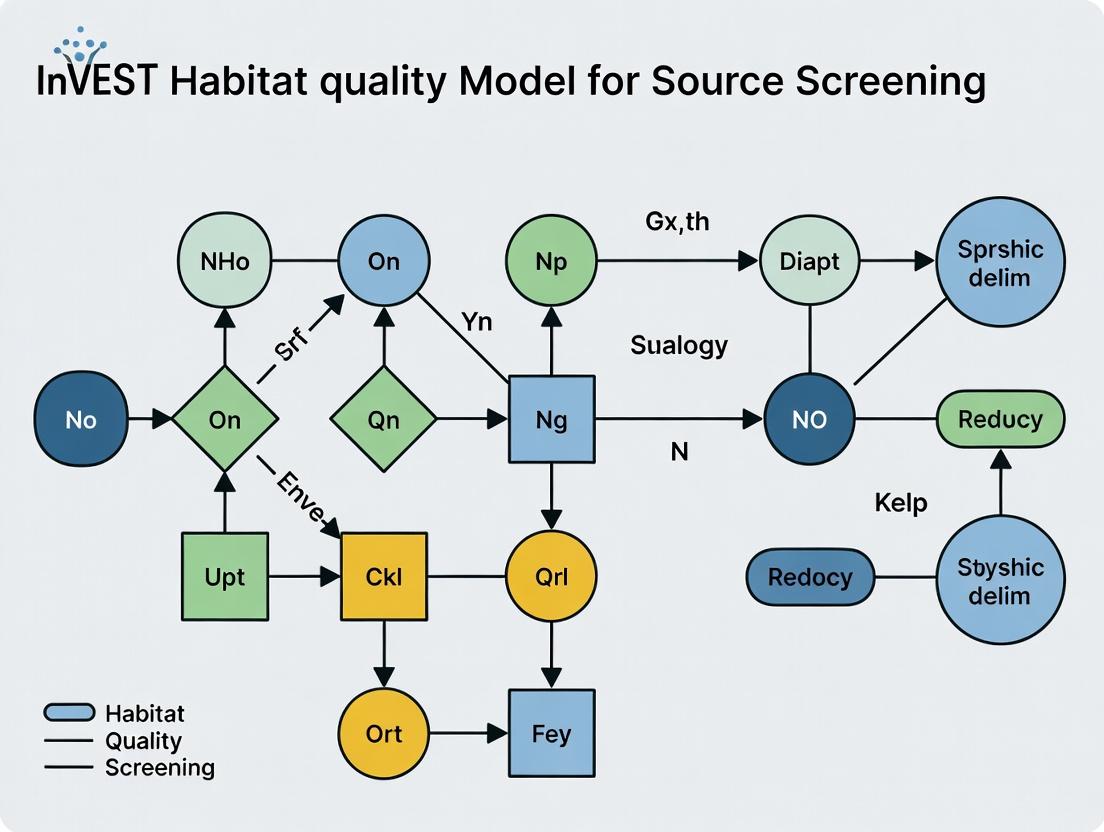
Title: InVEST Habitat Quality Model Logic for Source Screening
Title: Experimental Workflow for Model Calibration & Application
The Scientist's Toolkit
Table 3: Key Research Reagent Solutions & Materials
| Item | Function in Protocol/Modeling | Example/Specification |
|---|---|---|
| ICP-MS Standard Solutions | Calibration and quantification of trace metal contaminants in soil/plant samples during decay parameter validation. | Multi-element calibration standard (e.g., Cd, Pb, As, Cr). |
| Chlorophyll Fluorometer | Measures photosystem II efficiency (Fv/Fm) as a non-destructive, rapid assay of plant stress along threat gradients. | Portable PAM (Pulse-Amplitude Modulation) fluorometer. |
| Geographic Information System (GIS) Software | Platform for creating, managing, analyzing, and visualizing all spatial data layers (threats, habitat, output). | ArcGIS Pro, QGIS (open source). |
| InVEST Habitat Quality Model | The core software model that computationally integrates threat layers, sensitivity, and decay to produce degradation & quality maps. | Available from the Natural Capital Project (Stanford). |
| R or Python with Spatial Packages | For statistical analysis of field data, curve-fitting of decay functions, and advanced spatial analysis/scripting. | R (sf, raster), Python (geopandas, rasterio, scipy). |
| Expert Elicitation Database | A structured database (e.g., SQL, Excel) to manage, anonymize, and statistically analyze sensitivity scores from expert panels. | Custom-built with controlled entry forms. |
| Standardized Habitat Classification Scheme | Provides a consistent, defensible basis for defining habitat units and assigning sensitivities. | IUCN Global Ecosystem Typology, ESA CCI Land Cover. |
Application Notes
The integration of multi-scale biomedical data is a critical prerequisite for modern drug development and ecological modeling frameworks like the InVEST habitat quality model when applied to source screening for bioactive compounds. This convergence enables the systematic identification of promising molecular targets from natural or synthetic chemical libraries by evaluating their potential to perturb key biological networks.
Data Types and Their Role in Bio-Source Screening
Biomedical data provides the mechanistic layer that translates the "habitat quality" of a chemical source—its potential to yield high-value compounds—into testable biological hypotheses.
- Omics Data: Serves as the foundational phenotypic and molecular signature layer. Transcriptomics or proteomics profiles from diseased versus healthy tissues identify dysregulated genes/proteins, which become priority targets for intervention. In a source screening context, these targets are the "species" whose "habitat suitability" is being modeled.
- Pathway Databases: Provide the functional context, grouping disparate molecular targets into coherent biological processes (e.g., apoptosis, immune response). This allows researchers to move from single-target hits to pathway-level efficacy and toxicity predictions.
- Protein-Protein Interaction (PPI) Networks: Offer a systems-level view of cellular machinery. Essential proteins (hubs) in disease-associated PPI networks represent high-value, but potentially less obvious, therapeutic targets. Screening for compounds that modulate these hubs can be highly impactful.
Table 1: Key Public Data Sources for Biomedical Research Prerequisites
| Data Type | Primary Sources (Repository) | Typical Volume (as of 2024) | Primary Use in Screening |
|---|---|---|---|
| Genomics | NCBI dbSNP, gnomAD, TCGA | ~600 million human variants (gnomAD v4) | Identify genetic targets associated with disease risk. |
| Transcriptomics | GEO, ArrayExpress, GTEx | >150,000 curated series (GEO) | Discover differentially expressed gene targets & signatures. |
| Proteomics | PRIDE, Human Protein Atlas | >1 million mass spectrometry runs (PRIDE) | Validate protein-level target expression and modification. |
| Pathways | Reactome, KEGG, WikiPathways | ~2,400 human pathways (Reactome v86) | Contextualize targets and predict off-pathway effects. |
| PPI Networks | STRING, BioGRID, IntAct | ~2.5 million interactions (BioGRID 4.4) | Identify critical network hubs and multi-target strategies. |
Experimental Protocols
Protocol: Integrated Target Identification for Bio-Source Screening
Objective: To identify and prioritize high-confidence therapeutic targets from omics data within a biological pathway and network context, guiding the screening of compound sources.
Materials:
- Disease Gene Expression Dataset (e.g., from GEO: GSEXXXXX).
- Computational Tools: R/Python with limma/DESeq2 packages, Cytoscape.
- Reference Databases: KEGG/Reactome, STRING database.
Procedure:
- Differential Expression Analysis:
- Load normalized gene expression matrix and phenotype labels (e.g., Disease vs. Control) into R.
- Execute
DESeq2::DESeq()orlimma::lmFit()to perform statistical testing. - Apply a significance threshold (e.g., adjusted p-value < 0.05, \|log2 fold-change\| > 1). Export the list of differentially expressed genes (DEGs).
Pathway Enrichment Analysis:
- Input the DEG list into the
clusterProfiler::enrichKEGG()function in R. - Use default parameters (pAdjustMethod = "BH", pvalueCutoff = 0.05).
- Identify significantly enriched pathways. Select the top 5-10 pathways based on enrichment score and biological relevance to the disease.
- Input the DEG list into the
PPI Network Construction & Hub Gene Identification:
- Submit the DEG list to the STRING web API (confidence score > 0.7).
- Download the interaction file (TSV format) and import into Cytoscape.
- Run the CytoHubba plugin. Apply the Maximal Clique Centrality (MCC) algorithm to rank nodes.
- Select the top 10 hub genes from the ranked list.
Target Prioritization:
- Create a Venn diagram of genes appearing in DEGs, enriched pathways, and top hub genes.
- Genes in the intersection are considered high-priority targets for downstream in silico or in vitro screening of compound libraries.
Protocol:In SilicoCompound Screening Against Prioritized PPI Hubs
Objective: To screen a virtual compound library for potential binders against a prioritized protein hub target.
Materials:
- Target Protein Structure: PDB file (e.g., from RCSB PDB: 1ABC).
- Compound Library: SDF file of purchasable or natural compound collections (e.g., ZINC20 database subset).
- Software: AutoDock Vina or UCSF Chimera.
Procedure:
- Target Preparation:
- Load the PDB file into UCSF Chimera. Remove water molecules and heteroatoms. Add polar hydrogens and compute Gasteiger charges.
- Define the binding site grid box centered on known catalytic residues or literature-reported sites. Note the box center coordinates and dimensions.
Ligand Preparation:
- Convert the compound library SDF to PDBQT format using Open Babel:
obabel input.sdf -O ligands.pdbqt -m --gen3d.
- Convert the compound library SDF to PDBQT format using Open Babel:
Molecular Docking:
- Configure a Vina configuration file (
config.txt) specifying the receptor, ligand, and grid box parameters. - Execute batch docking:
vina --config config.txt --log results.log. - The output generates binding affinity estimates (in kcal/mol) for each ligand pose.
- Configure a Vina configuration file (
Hit Identification:
- Sort compounds by binding affinity (lower = stronger predicted binding). Apply a filter (e.g., affinity < -7.0 kcal/mol).
- Visually inspect the top 20-50 poses for favorable interactions (hydrogen bonds, hydrophobic packing). Select -10 top-ranked compounds for in vitro validation.
Visualizations
Diagram 1: Integrative Target Identification Workflow
Diagram 2: PI3K-Akt-mTOR Signaling Pathway
The Scientist's Toolkit
Table 2: Essential Research Reagents & Solutions for Omics and Network Analysis
| Item | Function/Application | Example Product/Resource |
|---|---|---|
| RNA Extraction Kit | Isolate high-integrity total RNA for transcriptomics (RNA-seq, microarrays). | Qiagen RNeasy Mini Kit, TRIzol Reagent. |
| Next-Generation Sequencing Library Prep Kit | Prepare fragmented and adapter-ligated DNA libraries for sequencing. | Illumina Nextera XT, NEBNext Ultra II. |
| Pathway Enrichment Software | Statistically identify biological pathways over-represented in a gene list. | clusterProfiler (R), GSEA software. |
| PPI Network Analysis Tool | Visualize and analyze protein interaction networks, identify hubs. | Cytoscape with STRING App. |
| Molecular Docking Suite | Predict binding orientation and affinity of small molecules to protein targets. | AutoDock Vina, Schrödinger Glide. |
| Curated Compound Library | Collection of annotated, drug-like molecules for virtual screening. | ZINC20 Database, ChEMBL. |
| Cell Viability Assay Kit | Validate screening hits by measuring compound toxicity or efficacy in vitro. | MTT Assay Kit, CellTiter-Glo. |
Step-by-Step Workflow: Building and Running an InVEST HQ Model for Target Prioritization
Within the thesis framework of applying the InVEST (Integrated Valuation of Ecosystem Services and Tradeoffs) habitat quality model to source screening in biomedical research, defining the biological 'landscape' is the critical first step. Analogous to mapping land cover types and habitat patches in ecology, this phase involves constructing a high-resolution, quantitative atlas of cell types, states, and spatial relationships within healthy and diseased tissues. This map serves as the foundational 'basemap' against which the 'sources' (e.g., novel drug targets, perturbed pathways) are later identified and prioritized for screening. This application note details modern protocols for building this biological context.
Key Quantitative Data Landscape
Table 1: Comparison of Single-Cell & Spatial Atlas Construction Platforms
| Platform/Technology | Typical Resolution | Throughput (Cells/Sample) | Key Measured Features | Primary Use Case in Context Building |
|---|---|---|---|---|
| 10x Genomics Chromium | Single-Cell | 1,000 - 10,000 cells | Gene expression (3’/5’), Immune repertoire, Surface proteins (Feature Barcode) | Unbiased cell type discovery and state characterization in dissociated tissues. |
| Nanostring GeoMx DSP | Regional (10-800µm ROI) | N/A (Region-based) | Whole Transcriptome or Protein (GeoMx) from user-defined tissue regions. | Profiling specific tissue microenvironments or morphological structures. |
| 10x Genomics Visium | Near-Single-Cell (55µm spots) | ~5,000 spots/slide | Whole Transcriptome with spatial context. | Mapping gene expression to tissue architecture without pre-selection. |
| Akoya CODEX/Phenocycler | Single-Cell (Spatial) | Millions of cells/whole slide | 40+ protein markers with subcellular resolution. | High-plex spatial phenotyping of cell types and cell-cell interactions. |
| BGI Stereo-seq | Subcellular (0.5µm bins) | Ultra-high density | Whole Transcriptome with high spatial fidelity. | Creating ultra-high resolution spatial atlases for fine tissue structuring. |
Table 2: Typical Cell-Type Composition in a Diseased Tissue Atlas (Example: Non-Small Cell Lung Cancer)
| Cell Type Cluster | % of Total Cells (Range) | Key Defining Markers (Human) | Putative Role in 'Habitat' |
|---|---|---|---|
| Malignant Epithelial | 20-60% | EPCAM+, KRT7+, Individual Clonotype | Core 'source' of dysregulation, driver of habitat alteration. |
| T Cells (Exhausted CD8+) | 5-25% | CD3E+, CD8A+, PDCD1+, LAG3+ | Immune response component, potential therapeutic target. |
| Tumor-Associated Macrophages | 10-30% | CD68+, CD163+, MRC1+ | Major component of immunosuppressive microenvironment. |
| Cancer-Associated Fibroblasts | 5-20% | ACTA2+, FAP+, COL1A1+ | Extracellular matrix remodeling, signaling hub. |
| Endothelial Cells | 2-10% | PECAM1+, VWF+, CDH5+ | Angiogenesis, nutrient/waste transport. |
| B Cells/Plasma Cells | 1-10% | CD79A+, MS4A1+, SDC1+ | Humoral immune response, antibody production. |
Experimental Protocols
Protocol 1: Generating a Single-Cell RNA-Seq Atlas from Diseased Tissue
Objective: To create a comprehensive, dissociated cell-type map of a tissue biopsy.
Materials: Fresh or preserved (in appropriate storage medium like RNAlater) tissue sample, dissociation enzyme cocktail (e.g., Miltenyi Biotec Tumor Dissociation Kit), PBS, viability dye (e.g., 7-AAD), cell strainer (70µm), 10x Genomics Chromium Controller & Single Cell 3’ Reagent Kits, Bioanalyzer/TapeStation.
Workflow:
- Tissue Dissociation: Mechanically mince tissue on ice. Incubate with optimized enzyme cocktail in a gentleMACS Dissociator or shaking water bath (37°C, 15-45 mins). Quench with complete media.
- Cell Suspension Preparation: Filter suspension through a 70µm strainer. Perform RBC lysis if needed. Wash cells twice with PBS + 0.04% BSA.
- Viability & Concentration Assessment: Count cells using a hemocytometer or automated counter. Assess viability with Trypan Blue or 7-AAD flow cytometry. Target viability >80%.
- Single-Cell Partitioning & Library Prep: Dilute cells to target concentration (700-1,200 cells/µl). Load onto 10x Chromium Chip B per manufacturer's instructions to generate Gel Bead-In-Emulsions (GEMs). Perform reverse transcription, cDNA amplification, and library construction using the Chromium Single Cell 3’ Reagent Kit v3.1.
- QC & Sequencing: Assess library quality (Bioanalyzer; expect peak ~450bp). Pool libraries and sequence on an Illumina platform (NovaSeq 6000). Target: ≥20,000 reads per cell.
Protocol 2: Spatial Transcriptomics Profiling with Visium
Objective: To map gene expression data onto tissue architecture.
Materials: Fresh-frozen tissue block, Cryostat, Visium Tissue Optimization Slide & Library Kit, Visium Spatial Gene Expression Slide, Fluorescent dyes, standard NGS reagents.
Workflow:
- Tissue Preparation: Section fresh-frozen tissue at 10µm thickness onto a Visium Spatial Gene Expression Slide. Perform H&E staining and imaging.
- Permeabilization Optimization: Using a separate Tissue Optimization slide, determine optimal tissue permeabilization time for maximal cDNA yield (range: 12-30 minutes).
- On-Slide cDNA Synthesis: For the main slide, perform tissue permeabilization (using optimized time), release and capture mRNA onto spatially barcoded primers on the slide. Synthesize cDNA in situ.
- Library Construction: Harvest cDNA from the slide, amplify, and fragment to construct sequencing libraries incorporating spatial barcodes.
- Sequencing & Data Integration: Sequence libraries. Use the spaceranger pipeline (10x Genomics) to align reads, count unique molecular identifiers (UMIs), and assign gene expression data to each spatial barcode spot, overlaying it with the H&E image.
Visualization of Workflows & Relationships
Diagram Title: Workflow for Constructing a Biological Context Atlas
Diagram Title: Target Signaling in Spatial Context
The Scientist's Toolkit: Research Reagent Solutions
Table 3: Essential Reagents for Biological Landscape Mapping
| Item | Function/Application | Example Product/Catalog |
|---|---|---|
| Tissue Dissociation Kit | Enzymatically dissociates solid tissues into viable single-cell suspensions for scRNA-seq. | Miltenyi Biotec, Human Tumor Dissociation Kit (130-095-929) |
| Viability Dye | Distinguishes live from dead cells during flow cytometry or sample QC prior to sequencing. | BioLegend, Zombie NIR Fixable Viability Kit (423106) |
| Single-Cell 3’ GEM Kit | Contains all reagents for partitioning cells, RT, and cDNA amplification on the 10x platform. | 10x Genomics, Chromium Next GEM Single Cell 3’ Kit v3.1 (1000121) |
| Visium Spatial Slide | Glass slide with ~5,000 barcoded spots for capturing mRNA from tissue sections. | 10x Genomics, Visium Spatial Gene Expression Slide (2000233) |
| Multiplex IHC Antibody Panel | Pre-validated antibodies for simultaneous imaging of 4-6 protein markers on one FFPE section. | Akoya Biosciences, Phenoptics Multiplex IHC Kits |
| Cell Hashing Antibody | Allows sample multiplexing (pooling) in scRNA-seq by labeling cells from different samples with distinct oligo-tagged antibodies. | BioLegend, TotalSeq-C Antibodies (e.g., Anti-Human Hashtag 1, 394661) |
| Nuclei Isolation Buffer | For extracting nuclei from frozen or hard-to-dissociate tissues for snRNA-seq. | 10x Genomics, Nuclei Isolation Kit (2000207) |
Within the InVEST (Integrated Valuation of Ecosystem Services and Tradeoffs) habitat quality model framework adapted for biomedical source screening, "Threats" represent disease drivers that degrade cellular or systemic functional integrity. This step quantifies the intensity and decay influence of three core threat categories—Genetic Variants, Epigenetic Modifications, and Environmental Exposures—on a target pathological endpoint. This quantification allows for the creation of a sensitivity-weighted threat map, prioritizing drivers for subsequent intervention screening.
Quantitative Data on Disease Drivers
Table 1: Prevalence and Effect Size of Key Genetic Drivers in Common Complex Diseases
| Disease | Key Genetic Loci (Example) | Risk Allele Frequency (%) | Odds Ratio (95% CI) | Heritability (%) |
|---|---|---|---|---|
| Alzheimer's Disease | APOE ε4 | ~15-25 (global) | 3.7 (3.3-4.1) | 58-79 |
| Type 2 Diabetes | TCF7L2 rs7903146 | ~30 (EUR) | 1.4 (1.34-1.47) | 30-70 |
| Coronary Artery Disease | 9p21 (CDKN2A/B) | ~50 (EUR) | 1.3 (1.25-1.35) | 40-60 |
| Rheumatoid Arthritis | HLA-DRB1 SE alleles | ~10-15 (EUR) | 4.6 (3.9-5.4) | 40-65 |
Table 2: Epigenetic Alterations Associated with Disease States
| Disease/Context | Epigenetic Marker | Target Loci/Region | Observed Change vs. Control | Quantification Method |
|---|---|---|---|---|
| Colorectal Cancer | DNA Methylation | SEPT9 Gene Promoter | Hypermethylation (>75% sensitivity) | MSP, qMSP |
| Metabolic Syndrome | Histone Modification | Hepatic PPARα | Reduced H3K27ac | ChIP-seq |
| Neuropsychiatric | DNA Hydroxymethylation | Brain-derived BDNF promoter | Decrease of 5hmC by ~30% | hMeDIP-seq |
| In Utero Smoke Exposure | DNA Methylation | AXL, PTPRO | Differential methylation (Δβ > 0.05) | 450K/EPIC Array |
Table 3: Environmental Exposure Metrics and Associated Disease Risk
| Exposure Factor | Typical Quantitative Measure | Associated Health Outcome | Increased Relative Risk (RR) per Unit Increase |
|---|---|---|---|
| PM2.5 Air Pollution | Annual mean (μg/m³) | All-cause mortality | RR 1.08 per 10 μg/m³ |
| Dietary Sodium | 24h Urinary Na (g/day) | Cardiovascular Events | RR 1.18 per 2.5g/day |
| Chronic Psychosocial Stress | Perceived Stress Scale (PSS) Score | Major Depression | OR 1.5 per SD increase |
| Aflatoxin B1 | Biomarker (AFB1-Lys in serum) | Hepatocellular Carcinoma | RR 1.3 per log unit |
Detailed Experimental Protocols
Protocol 1: Genome-Wide Association Study (GWAS) for Genetic Threat Quantification
Objective: Identify and quantify the effect size of single nucleotide polymorphisms (SNPs) associated with a disease phenotype.
Materials: Case-control cohort DNA samples, SNP microarray chips (e.g., Illumina Global Screening Array), high-throughput genotyping platform, bioinformatics software (PLINK, SNPTEST).
Procedure:
- Sample & QC: Isolate high-quality genomic DNA from cases (disease) and matched controls. Quality control (QC): spectrophotometric quantification (A260/A280 ~1.8), agarose gel check for degradation.
- Genotyping: Perform genome-wide genotyping per manufacturer's protocol. Standardize intensities and cluster genotypes for each SNP.
- Data QC: Filter samples for call rate >98%, gender inconsistencies, heterozygosity outliers, and population stratification (via PCA). Filter SNPs for call rate >95%, minor allele frequency (MAF) >1%, and Hardy-Weinberg equilibrium (p > 1x10⁻⁶ in controls).
- Association Analysis: Perform logistic regression for each SNP, adjusting for covariates (age, sex, principal components). Calculate odds ratios (OR) and p-values.
- Significance & Validation: Apply genome-wide significance threshold (p < 5x10⁻⁸). Replicate top hits in an independent cohort. Quantify threat via OR and population attributable fraction.
Protocol 2: Epigenome-Wide Association Study (EWAS) Using Methylation Arrays
Objective: Identify differentially methylated CpG sites associated with an environmental exposure or disease state.
Materials: Bisulfite conversion kit (e.g., EZ DNA Methylation Kit), Infinium MethylationEPIC BeadChip, iScan system, bioinformatics tools (R package minfi, ChAMP).
Procedure:
- Bisulfite Conversion: Treat 500ng genomic DNA with sodium bisulfite, converting unmethylated cytosines to uracil (methylated cytosines remain unchanged). Purify converted DNA.
- Microarray Processing: Amplify, fragment, and hybridize bisulfite-converted DNA to the BeadChip. Perform single-base extension and fluorescent staining on the iScan scanner.
- Data Preprocessing: Extract intensity data (idat files). Perform normalization (e.g., SWAN, Noob), and probe filtering (remove cross-reactive, SNP-containing probes). Calculate β-values (methylation level, range 0-1) for each CpG.
- Statistical Analysis: Fit a linear regression model (or a mixed model for complex designs) for each CpG, with β-value as outcome and exposure/disease status as predictor, adjusting for cell type composition (Houseman method), age, sex, and batch effects.
- Threat Quantification: Identify significant CpGs (FDR < 0.05). Calculate Δβ (mean difference) and report as percentage point change. Annotate to genomic features (promoter, enhancer, gene body).
Protocol 3: High-Resolution Environmental Exposure Biomarker Profiling (Liquid Chromatography-Tandem Mass Spectrometry)
Objective: Quantify specific chemical exposure metabolites (xenobiotics) in human biospecimens.
Materials: Serum/urine samples, internal standards (isotope-labeled), solid-phase extraction (SPE) columns, UPLC system coupled to triple quadrupole MS (e.g., Waters Xevo TQ-S), analytical columns (C18).
Procedure:
- Sample Preparation: Thaw samples on ice. Add isotopically labeled internal standard to correct for recovery and matrix effects. Precipitate proteins (e.g., with cold acetonitrile) or perform SPE for cleanup. Evaporate and reconstitute in mobile phase.
- LC-MS/MS Method: Inject sample onto UPLC column. Use a gradient of water and acetonitrile (both with 0.1% formic acid) for separation. Elute analytes into the MS.
- Mass Spectrometry: Operate in multiple reaction monitoring (MRM) mode. Optimize source parameters (capillary voltage, desolvation temperature) and compound-specific collision energies for parent→product ion transitions.
- Calibration & Quantification: Run a calibration curve with known concentrations of the analyte alongside samples. Use the ratio of analyte peak area to internal standard peak area to calculate concentration from the linear regression of the calibration curve.
- Data Analysis: Express exposure as concentration (e.g., ng/mL). Correlate with clinical endpoints using statistical models, calculating threat as the beta coefficient or hazard ratio per interquartile range increase in exposure.
Signaling Pathway & Workflow Visualizations
Diagram 1: Threat Quantification in InVEST Biomedical Model
Diagram 2: Epigenome-Wide Association Study Protocol
The Scientist's Toolkit: Research Reagent Solutions
Table 4: Essential Reagents & Kits for Threat Quantification Experiments
| Item Name (Example) | Vendor (Example) | Primary Function in Protocol |
|---|---|---|
| DNeasy Blood & Tissue Kit | Qiagen | High-yield, high-purity genomic DNA extraction for GWAS/EWAS. |
| Infinium MethylationEPIC Kit | Illumina | Genome-wide profiling of >850,000 CpG methylation sites for EWAS. |
| EZ-96 DNA Methylation-Gold Kit | Zymo Research | Reliable bisulfite conversion of DNA for downstream methylation analysis. |
| TaqMan SNP Genotyping Assays | Thermo Fisher | High-throughput, accurate allelic discrimination for SNP validation. |
| Mass Spectrometry Grade Solvents | Sigma-Aldrich | Low-UV absorbance, high-purity solvents for LC-MS/MS exposure profiling. |
| Certified Reference Standards (Serum) | NIST | Calibrators and controls for quantitative accuracy in exposure assays. |
| ChIP-Grade Antibodies (e.g., H3K27ac) | Abcam | Specific immunoprecipitation of histone modifications for ChIP-seq. |
| NucleoSpin Plasma XS Kit | Macherey-Nagel | Efficient extraction of cell-free DNA for liquid biopsy-based analyses. |
Application Notes Within the InVEST habitat quality model framework for source screening (e.g., identifying bioactive natural product sources), assigning "sensitivity" is analogous to determining a biological target's vulnerability or a pathogen's susceptibility. This step quantifies the potential impact of a "threat" (e.g., a compound) on a "habitat" (e.g., a cancer cell or microbial pathogen). This protocol details the curation of target- or pathogen-specific sensitivity scores from biomedical literature and databases to parameterize this component of the model, enabling prioritization of source organisms based on the predicted potency of their putative metabolites.
Experimental Protocol: Sensitivity Score Curation Workflow
1. Objective: To compile and standardize quantitative vulnerability metrics (e.g., IC₅₀, Minimum Inhibitory Concentration (MIC), Essentiality Scores) for predefined biological targets or pathogens of interest from public resources.
2. Materials & Databases:
- Primary Scientific Literature (PubMed, Google Scholar)
- Target-Specific Databases: ChEMBL, BindingDB, The Cancer Dependency Map (DepMap)
- Pathogen-Specific Databases: CARD (Comprehensive Antibiotic Resistance Database), EUCAST, PubMed Central
- Data Management Software: Microsoft Excel, Python/R for data wrangling, Zotero/EndNote
3. Procedure:
A. Define Search Strategy & Criteria:
- For each target/pathogen, formulate a Boolean search string. Example:
"(Target X OR Gene Symbol Y) AND (inhibition IC50 OR knockdown) AND (cancer cell line Z)"or"(Pathogen name) AND (MIC) AND (natural product)". - Set inclusion/exclusion criteria: species (e.g., human vs. murine), assay type (e.g., biochemical vs. cellular), publication date (prioritize last 10 years).
B. Systematic Data Extraction:
- Execute searches in the listed databases. Screen titles/abstracts for relevance.
- From selected full-text articles, extract the following into a standardized template:
- Target/Pathogen Name
- Perturbation Agent (Compound/Gene)
- Quantitative Metric (IC₅₀, MIC, Gene Effect Score)
- Unit (nM, µg/mL, etc.)
- Assay System (e.g., cell line, strain)
- PubMed ID (PMID)
C. Data Normalization & Scoring:
- Convert all concentration-based metrics (IC₅₀, MIC) to a logarithmic scale (pIC₅₀ = -log₁₀(IC₅₀ in Molars); pMIC = -log₁₀(MIC in g/L)) to normalize the distribution.
- For genetic dependency scores (e.g., from DepMap), use the publicly available CERES or Chronos gene effect scores directly, where more negative scores indicate higher essentiality/vulnerability.
- For a given target/pathogen, calculate the median normalized score from all curated data points. This median becomes the Sensitivity Score (S) for model input. A higher score indicates greater vulnerability.
D. Confidence Assessment:
- Assign a Data Confidence Code (1-3) based on data concordance and source reliability.
- Code 1 (High): Consensus from multiple high-quality studies or a public database benchmark.
- Code 2 (Medium): Data from a few studies with some variability in reported values.
- Code 3 (Low): Data from a single, preliminary study.
4. Data Presentation: Curated Sensitivity Scores Table
Table 1: Example Curated Sensitivity Scores for Model Parameterization
| Target / Pathogen | Sensitivity Score (S) | Score Type | Raw Value Median | Data Confidence | Key Database/Source |
|---|---|---|---|---|---|
| Target: HSP90AA1 | 7.52 | pIC₅₀ | 30 nM | 1 (High) | ChEMBL, 3+ studies |
| Target: EGFR (L858R) | 8.00 | pIC₅₀ | 10 nM | 1 (High) | BindingDB, Clin. data |
| Pathogen: S. aureus (MRSA) | 2.15 | pMIC | 7.1 µg/mL | 2 (Medium) | PubMed (5 studies) |
| Gene: MYC (in PANC-1) | -0.92 | CERES Score | -0.92 | 1 (High) | DepMap (22Q4) |
Diagram: Sensitivity Score Curation Workflow
Sensitivity Score Data Pipeline
The Scientist's Toolkit: Key Research Reagent Solutions
Table 2: Essential Materials for Sensitivity Data Curation
| Item | Function in Protocol |
|---|---|
| ChEMBL Database | Public repository of bioactive molecules with curated binding/functional data for target-based sensitivity scoring. |
| DepMap Portal | Provides genome-wide CRISPR knockout screens yielding quantitative gene essentiality (vulnerability) scores. |
| Zotero Reference Manager | Collects, manages, and cites literature from database searches; enables team-based curation. |
| Python Pandas Library | For scripting the normalization, filtering, and statistical summarization (median calculation) of extracted data. |
| EUCAST MIC Distributions | Standardized data for epidemiological cutoff values to contextualize pathogen MIC sensitivity scores. |
Within the broader thesis applying the InVEST (Integrated Valuation of Ecosystem Services and Tradeoffs) habitat quality model to source screening for drug target identification, this step is critical. The InVEST model traditionally quantifies how habitat quality decays with distance from a "source" habitat patch, factoring in resistance from the landscape matrix. In biological network analysis for drug development, we analogously model how influence (e.g., a signal, perturbation, or therapeutic effect) propagates from a source node (e.g., a drug target). The "landscape" is the network topology. Configuring decay parameters defines the rate of signal attenuation over network distance, while accessibility parameters account for the varying resistance of different node types or edge weights to influence flow. This step translates ecological principles into a computational framework for predicting downstream effects and off-target interactions in cellular systems.
Core Parameter Definitions & Quantitative Data
The propagation of influence from a source node s to a target node t is modeled as a decaying function of the effective distance d(s,t). The following table summarizes the key configurable parameters and their typical value ranges derived from current literature.
Table 1: Core Decay and Accessibility Parameters for Influence Propagation
| Parameter | Symbol | Description | Typical Range / Value | Biological/Network Analogy |
|---|---|---|---|---|
| Base Decay Rate | β | The constant rate at which influence diminishes per unit of network distance. | 0.1 - 0.8 | Signal transduction efficiency; enzymatic reaction rate. |
| Distance Metric | d(s,t) | The measure of path length between nodes. | Shortest Path, Diffusive Path, Random Walk | Metabolic steps; signaling cascade length. |
| Decay Function | f(d) | Mathematical function mapping distance to influence level. I(t) = I₀ * f(d). | Exponential: e^(-βd) Power-Law: d^(-γ) Threshold: 1 if d ≤ D, 0 if d > D | Protein binding affinity decay; pharmacological effect decay. |
| Exponent (Power-Law) | γ | Sensitivity of decay to distance in power-law models. | 1.0 - 3.0 | Scale-free network connectivity distribution. |
| Threshold Distance | D | Maximum effective propagation distance. | 2 - 5 steps | Limited cascade depth in canonical pathways. |
| Edge Resistance Weight | r(e) | Resistance to influence flow on edge e (inverse of weight). | Normalized [0, 1] or [1, ∞) | Interaction strength (Kd, Km); confidence score. |
| Node Accessibility Factor | α(n) | Node-specific modifier for receiving/integrating influence. | 0.0 (blocked) - 1.5 (amplifier) | Node degree, centrality, or functional state (e.g., mutated, expressed). |
Experimental Protocols for Parameter Calibration
Protocol 3.1: Calibrating Decay Rate (β) Using Phospho-Proteomics Time-Series Data
Objective: Empirically determine the base decay rate β for a specific signaling network by fitting an exponential decay model to time-resolved phosphorylation data following pathway stimulation.
Materials: Cultured cell line, pathway-specific agonist/antagonist, LC-MS/MS platform, phospho-specific antibodies, network model (e.g., from STRING or KEGG).
Procedure:
- Stimulation & Sampling: Apply a precise stimulus (e.g., EGF ligand) to cells at t=0. Collect cell lysates at multiple time points (e.g., 0, 2, 5, 15, 30, 60 min).
- Quantitative Measurement: Use targeted mass spectrometry or high-throughput immunoassays to quantify phosphorylation levels of key proteins in the pathway of interest. Normalize data to t=0.
- Network Distance Mapping: For each measured protein (node t), calculate its shortest path distance d from the primary receptor (source node s) in the curated network.
- Data Fitting: For each time point, plot the normalized phosphorylation level (I/I₀) against network distance d. Fit the data to the exponential decay model: I/I₀ = e^(-β(t) * d), where β(t) is the time-dependent decay rate.
- Parameter Extraction: The decay rate β for steady-state influence propagation is typically taken as the asymptotic value of β(t) at later time points (e.g., t=60 min). Perform nonlinear regression to obtain the optimal β.
Protocol 3.2: Determining Edge Resistance Weights (r(e)) via Integration of Multi-Omics Data
Objective: Derive biologically informed edge resistance weights for a protein-protein interaction (PPI) network to model differential influence propagation.
Materials: Base PPI network (BioGRID, IntAct), gene expression dataset (e.g., RNA-Seq from relevant tissue), protein-protein affinity data (if available), computational platform (e.g., Cytoscape, custom Python/R scripts).
Procedure:
- Network Pruning: Start with a high-confidence PPI network. Remove interactions not supported in the biological context of interest (e.g., filter by co-expression, using a correlation threshold > 0.7).
- Weight Assignment: For each remaining edge e between proteins i and j, compute a composite weight w(e). A proposed formula is: w(e) = (CI_ij * (EX_i + EX_j)/2)^k, where CI is a confidence score from the database, EX is normalized expression level, and k is a scaling constant (often 1).
- Convert to Resistance: Compute edge resistance as the inverse of the normalized weight: r(e) = 1 / (w(e) + ε), where ε is a small constant to prevent division by zero.
- Validation: Simulate perturbation propagation using the weighted network and compare predicted key influencer nodes to essential genes from CRISPR knockout screens. Iteratively adjust the weighting formula to maximize concordance.
Visualization of Concepts and Workflows
Diagram 1: Influence Propagation with Decay & Accessibility
Diagram 2: Parameter Calibration Workflow
The Scientist's Toolkit: Research Reagent Solutions
Table 2: Essential Materials for Propagation Modeling & Calibration
| Item / Reagent | Function in Protocol | Example Product / Resource |
|---|---|---|
| Pathway-Specific Bioactive Ligands | To provide a controlled, potent stimulus at the defined source node for calibration experiments. | Recombinant human EGF (BioTechne), SAG (Smoothened Agonist) (Tocris). |
| Phospho-Specific Antibody Panels | To quantify activation/influence levels of multiple network nodes (proteins) simultaneously via immunoassays. | Phospho-MAPK Array Kit (R&D Systems), TotalSeq Antibodies (BioLegend) for CITE-seq. |
| Tandem Mass Tag (TMT) Reagents | For multiplexed, quantitative global phospho-proteomics to measure signaling dynamics network-wide. | TMTpro 16plex Label Reagent Set (Thermo Fisher Scientific). |
| CRISPR Knockout Pooled Libraries | To generate validation data on node essentiality and functional influence for model tuning. | Brunello Human Whole Genome CRISPR Knockout Library (Addgene). |
| Curated Network Databases | Provide the initial topological scaffold (nodes/edges) for building the propagation model. | STRING, KEGG, Reactome, SIGNOR. |
| Network Analysis & Simulation Software | Platform to implement decay/accessibility rules, run propagation simulations, and fit parameters. | Cytoscape with DyNet plugin, Python (NetworkX, NDEx2), R (igraph, influenceR). |
| Nonlinear Regression Tools | To fit exponential/power-law decay models to experimental distance-response data. | GraphPad Prism, Python SciPy.optimize.curve_fit, R nls(). |
Within the broader thesis applying the InVEST (Integrated Valuation of Ecosystem Services and Tradeoffs) Habitat Quality model to drug target screening, Step 5 represents the translational pivot. This phase operationalizes the model's output—a spatially explicit Habitat Quality (HQ) score—by reinterpreting it as a Target Priority Index (TPI). The core analogy maps ecological concepts to pharmacological research: high-quality habitat patches equate to high-priority biological targets, threat sources equate to disease drivers, and threat sensitivity equates to target vulnerability or mechanistic relevance. This protocol details the execution, calibration, and interpretation of the model for this novel application.
Core Data & Parameter Translation Tables
The model requires the translation of biological and pharmacological data into InVEST-compatible spatial layers. The tables below summarize key quantitative inputs and outputs.
Table 1: Input Data Layer Translation for Target Screening
| InVEST Layer | Biological Analog | Data Source Examples | Format & Key Metrics |
|---|---|---|---|
| Land Use/Land Cover (LULC) | Target Universe Map | - OMIM database- GTEx tissue atlas- Protein Atlas- CRISPR screening hits | Raster/Vector. Each pixel/cell represents a potential target (e.g., gene, protein). Classes define target types (e.g., GPCRs, kinases, ion channels). |
| Threat Sources | Disease Drivers | - Genomic (GWAS loci)- Transcriptomic (dysregulated pathways)- Proteomic (aberrant protein activity)- Metabolomic (pathway fluxes) | Raster/Vector. Intensity based on effect size (β, odds ratio), fold-change, or pathway enrichment score (p-value). |
| Threat Sensitivity | Target Vulnerability | - Essentiality scores (DepMap)- Pathway centrality | Table (.csv). Sensitivity (0-1) per target type to each disease driver, derived from literature mining and bioinformatics. |
| Accessibility | 'Druggability' Modifier | - Protein structure (PDB)- Ligandability assays- Existing pharmacopeia | Raster. Distance decay based on structural feasibility, chemical tractability, and competitive landscape. |
Table 2: Model Output Interpretation: HQ Score to TPI
| HQ Score Range | Interpretation (Ecological) | Translated TPI Priority | Recommended Action |
|---|---|---|---|
| 0.8 - 1.0 | Very High Quality Habitat | Very High Priority Target | Immediate validation; high confidence for therapeutic intervention. |
| 0.6 - 0.8 | High Quality Habitat | High Priority Target | Strong candidate for in vitro/in vivo functional studies. |
| 0.4 - 0.6 | Moderate Quality Habitat | Moderate Priority Target | Context-dependent validation; consider for combination strategies. |
| 0.2 - 0.4 | Low Quality Habitat | Low Priority Target | Deprioritize unless supported by orthogonal evidence. |
| 0.0 - 0.2 | Very Low/ Degraded Habitat | Very Low Priority | Likely poor or high-risk target; exclude from shortlist. |
Experimental Protocols for Model Calibration & Validation
Protocol 3.1: Calibrating Threat Sensitivity Scores via CRISPR-Cas9 Functional Genomics Objective: To empirically derive threat sensitivity values for target classes (e.g., kinases) against a specific disease driver (e.g., oncogenic signaling). Materials: See "Scientist's Toolkit" below. Method:
- Cell Line Selection: Choose a disease-relevant cell line (e.g., a cancer cell line with a defined oncogenic driver).
- CRISPR Library: Employ a targeted sgRNA library focusing on the target class of interest (e.g., kinome-wide library).
- Proliferation Screen: Conduct a pooled CRISPR knockout screen under baseline and driver-activated conditions (e.g., with/ without cytokine stimulation). Include non-targeting control sgRNAs.
- Differential Analysis: Calculate gene-level fitness scores (e.g., MAGeCK MLE) for both conditions.
- Sensitivity Score Calculation: For each gene i, compute a normalized sensitivity score S_i: S_i = (FitnessScoreDriverOn - FitnessScore_Baseline) / max(|Δ| across all genes). Clamp values to [0,1], where 1 indicates maximal vulnerability to the driver.
- Class Aggregation: Average S_i scores for all genes within a defined target class (e.g., all tyrosine kinases) to generate the class-level sensitivity parameter for the model.
Protocol 3.2: Validating TPI with High-Throughput Compound Screening Objective: To assess if targets with higher TPI scores show greater response to pharmacological modulation in a phenotypic assay. Materials: See "Scientist's Toolkit." Method:
- Target Selection: Select a panel of 4-6 targets spanning the TPI range (e.g., High, Medium, Low).
- Perturbation: Use siRNA/shRNA (knockdown) or selective small-molecule inhibitors (where available) for each target.
- Phenotypic Assay: Perform a disease-relevant high-content assay (e.g., cell viability, apoptosis, reporter activity) in a driver-positive cellular model.
- Dose-Response: Test each perturbation across a minimum of 8 concentration points in triplicate.
- Analysis: Calculate Z-scores for effect size and IC50/EC50 values.
- Validation Correlation: Perform Spearman correlation analysis between the in silico TPI scores for the selected targets and their corresponding phenotypic effect Z-scores (or -log10(IC50)). A significant positive correlation (p < 0.05) validates the model's predictive power.
Visualizing the TPI Workflow & Logic
Title: Workflow from Biological Data to Target Priority Decision
The Scientist's Toolkit: Research Reagent Solutions
| Item | Function in TPI Framework | Example Product/Resource |
|---|---|---|
| CRISPR Knockout Library | Generates empirical data for calibrating threat sensitivity scores. | Addgene: Brunello whole-genome or custom sub-libraries (e.g., kinome). |
| High-Content Screening System | Enables phenotypic validation of TPI predictions via multiplexed assay readouts. | PerkinElmer Operetta or Molecular Devices ImageXpress. |
| Selective Small-Molecule Inhibitors | Tools for pharmacological perturbation of high-TPI targets in validation assays. | Tocris Bioscience or Selleckchem inhibitor libraries. |
| siRNA/shRNA Reagents | Allows rapid knockdown of target genes for functional validation. | Horizon Discovery siGENOME or Sigma-Aldrich MISSION shRNA. |
| Bioinformatics Suites | For processing omics data into threat rasters and analyzing model outputs. | Qiagen IPA, Partek Flow, or custom R/Python pipelines. |
| InVEST Software | The core modeling platform for executing the habitat quality algorithm. | Natural Capital Project InVEST (version 3.14 or later). |
Common Pitfalls and Advanced Optimization Strategies for Robust Screening
Troubleshooting Data Gaps and Heterogeneity in Biomedical Threat Layers
1. Introduction and Thesis Context Within the framework of a broader thesis employing the InVEST Habitat Quality model for source screening in biomedical threat discovery, the integrity of input "threat layers" is paramount. These layers, analogous to habitat degradation sources, represent quantified biomedical risks (e.g., zoonotic host prevalence, antimicrobial resistance gene abundance, pathogen environmental persistence). Data gaps (missing values) and heterogeneity (incompatible formats, scales, or collection methodologies) directly propagate as uncertainty in model outputs, compromising the identification of high-priority threats. This document provides application notes and protocols for diagnosing and mitigating these data challenges.
2. Quantifying Data Gaps and Heterogeneity: A Diagnostic Table A systematic audit of threat layers is the essential first step. The following metrics should be calculated per layer.
Table 1: Diagnostic Metrics for Threat Layer Assessment
| Metric | Calculation | Interpretation |
|---|---|---|
| Spatial Coverage Gap (%) | (Number of missing grid cells / Total grid cells) * 100 | >5% may require imputation or mask application. |
| Temporal Completeness | Time series continuity score (e.g., % of months with data over study period). | Discontinuities can introduce seasonal bias. |
| Scale Heterogeneity Index | Coefficient of Variation (CV) across datasets merged into the layer. | CV > 30% indicates high variability requiring normalization. |
| Methodological Discordance | Categorical score (1-5) based on divergence in source collection protocols. | Scores ≥3 necessitate cross-walk functions or uncertainty layers. |
| Detection Limit Impact | % of values at the assay's lower limit of detection (LLOD). | High LLOD% may bias low-end values upward. |
3. Experimental Protocols for Data Harmonization
Protocol 3.1: Geospatial Imputation for Coverage Gaps
Objective: To estimate missing values in a spatially correlated threat layer (e.g., soil pathogen load).
Materials: GIS software (e.g., QGIS, ArcGIS), R/Python with gstat or raster packages.
Procedure:
- Diagnostic Mapping: Visualize the spatial distribution of missing data (gaps).
- Variogram Modeling: Calculate an empirical variogram to model spatial autocorrelation.
- Kriging Interpolation: Apply ordinary kriging using the fitted variogram model to predict values at missing locations.
- Uncertainty Quantification: Generate the kriging variance layer to annotate imputed areas with higher uncertainty.
- Validation: If data permits, withhold 10% of known points pre-imputation to validate prediction error (RMSE).
Protocol 3.2: Cross-Walk Calibration for Methodological Heterogeneity Objective: To align two datasets measuring the same threat (e.g., seroprevalence) but using different assays. Materials: Reference standard samples, statistical software (R, Stata). Procedure:
- Paired Sample Testing: Assay a panel of n≥30 reference samples covering the measurement range with both Method A (legacy) and Method B (new).
- Regression Modeling: Fit a linear or non-linear (e.g., Deming) regression:
Method_B = β0 + β1 * Method_A + ε. - Cross-Walk Function: Derive the formula to convert values from Method A to the scale of Method B.
- Apply & Flag: Convert all legacy data using the cross-walk function. Create a metadata flag indicating conversion.
4. Visualization of Data Integration Workflow
Diagram Title: Threat Layer Harmonization Workflow for InVEST
5. The Scientist's Toolkit: Research Reagent Solutions
Table 2: Essential Tools for Threat Layer Construction and Harmonization
| Item / Reagent | Function in Threat Layer Research |
|---|---|
| Synthetic Standard Panels | Provides a calibrated reference for cross-assay comparison and cross-walk development (e.g., for pathogen genomic load quantification). |
| Geo-Referenced Biobank Samples | Enables ground-truthing of spatially imputed data and validation of environmental threat layers. |
| Uniform Data Collection Kits | Standardized sampling swabs, buffers, and protocols reduce methodological heterogeneity at source. |
| Open-Source Data Cubes | Pre-processed, analysis-ready data (e.g., NASA SEDAC, Earth Engine) provide consistent baselines for spatial modeling. |
| Uncertainty Quantification Software | Libraries (e.g., PyMC3, gstat) propagate measurement and imputation error through to final model outputs. |
Within the framework of InVEST (Integrated Valuation of Ecosystem Services and Trade-offs) habitat quality model source screening for drug discovery, sensitivity scores traditionally categorize the ecological threat of pharmaceutical compounds and their metabolites as static, binary annotations (e.g., high/low). This static approach fails to capture the dynamic, context-dependent nature of biological activity. This document outlines protocols to calibrate these sensitivity scores by integrating dynamic biochemical context—specifically, protein binding affinity, metabolic transformation pathways, and cellular stress response signaling—to generate a more predictive, mechanism-based risk assessment for environmental source screening.
Key Experimental Protocols
Protocol 2.1: Dynamic Contextualization of Compound Sensitivity via Protein-Ligand Interaction Profiling
- Objective: To measure binding affinity (Kd) of a target compound and its major metabolites against a panel of conserved eukaryotic proteins (e.g., cytochrome P450 isoforms, HSP90, ion channels).
- Materials: See Scientist's Toolkit.
- Procedure:
- Sample Preparation: Recombinantly express and purify target proteins. Prepare a dilution series of the test compound (parent and Phase I metabolites) in assay buffer.
- Microscale Thermophoresis (MST):
- Label the target protein using a fluorescent dye kit.
- Mix constant concentrations of labeled protein with the compound dilution series.
- Load samples into premium coated capillaries.
- Perform MST measurements using a Monolith series instrument. The laser induces a temperature gradient, and the fluorescence change is monitored.
- Fit the dose-response curve using the instrument software to calculate the Kd for each compound-protein pair.
- Data Integration: Normalize Kd values to a log scale. Integrate with InVEST by creating a dynamic "binding sensitivity score" modifier, where lower Kd (higher affinity) proportionally increases the base static sensitivity score for the compound.
Protocol 2.2: Mapping Metabolic Activation Pathways to Stress Signaling Crosstalk
- Objective: To experimentally link compound metabolism to the activation of specific stress response pathways in a model hepatic cell line.
- Materials: HepG2 cells, LC-MS/MS, qPCR reagents, pathway-specific inhibitors/activators.
- Procedure:
- Treatment & Metabolite Profiling: Treat HepG2 cells with the compound of interest (e.g., 10µM, 24h). Extract intracellular metabolites. Perform untargeted LC-MS/MS to identify major Phase I and II metabolites.
- Pathway Activation Reporter Assay: Co-transfect HepG2 cells with reporters for key pathways: Antioxidant Response Element (ARE), NF-κB Response Element, and p53 Response Element.
- Treat transfected cells with the parent compound and identified key reactive metabolites.
- Measure luciferase activity to quantify pathway-specific activation.
- Validation via qPCR: Isolate RNA from treated cells. Perform qPCR for canonical markers of each activated pathway (e.g., HMOX1 for ARE, IL8 for NF-κB, CDKN1A for p53).
- Contextual Score: The number and magnitude of significantly activated stress pathways generate a "contextual stress multiplier" for the base sensitivity score.
Data Presentation
Table 1: Comparison of Static vs. Dynamically Calibrated Sensitivity Scores for Model Compounds
| Compound (Parent) | Static InVEST Score | Key Metabolite Identified | Primary Protein Target (Kd, nM) | Dominant Stress Pathway Activated | Calibrated Dynamic Score | % Change from Static |
|---|---|---|---|---|---|---|
| Model Drug A | 0.75 (High) | Quinone-imine | KEAP1 (15.2 ± 2.1) | ARE (8.5-fold) | 0.92 | +22.7% |
| Model Drug B | 0.40 (Moderate) | N-acetyl cysteine adduct | CYP3A4 (2100 ± 310) | NF-κB (3.2-fold) | 0.55 | +37.5% |
| Model Drug C | 0.80 (High) | None (parent stable) | HSP90 (85.7 ± 9.4) | p53 (1.8-fold) | 0.83 | +3.8% |
Table 2: Research Reagent Solutions Toolkit
| Item/Category | Product Example/Description | Primary Function in Calibration Protocols |
|---|---|---|
| Protein Purification System | HisTrap HP column, AKTA system | Isolation of recombinant target proteins for binding assays. |
| Microscale Thermophoresis (MST) Instrument | Monolith X | Precisely measures binding affinity (Kd) between compounds and target proteins in solution. |
| Fluorescent Labeling Kit | Protein Labeling Kit RED-NHS 2nd Generation | Covalently labels purified proteins for MST detection. |
| Hepatic Cell Line | HepG2 (ATCC HB-8065) | In vitro model for studying compound metabolism and cellular stress response. |
| Pathway Reporter Assay | Cignal Lenti Reporter (ARE, NF-κB, p53) | Quantifies transcriptional activation of specific stress signaling pathways. |
| Metabolite Profiling Platform | Q-TOF LC-MS/MS System (e.g., Agilent 6546) | Identifies and characterizes Phase I/II metabolites from biological samples. |
Mandatory Visualizations
Dynamic Sensitivity Calibration Workflow
ARE Stress Pathway Activation by Metabolites
Optimizing Decay Parameters (Linear vs. Exponential) for Biological Signal Propagation
Within the framework of a broader thesis employing the InVEST (Integrated Valuation of Ecosystem Services and Tradeoffs) habitat quality model for ecological source screening, this protocol addresses a parallel challenge in in vitro biological systems: quantifying signal propagation from a source. The InVEST model uses decay functions (linear and exponential) to model the degradation of habitat quality as a function of distance from a pollution source. This concept is directly analogous to modeling the decay of a biological signal (e.g., cytokine concentration, electrical potential) as it propagates from a cellular source through a medium or tissue. Optimizing the decay parameter (k) for linear (signal = max - kdistance) vs. exponential (signal = max * e^(-kdistance)) models is critical for accurately predicting effective biological activity ranges in drug delivery, chemotaxis studies, and microenvironment mapping.
Table 1: Comparative Properties of Linear vs. Exponential Decay Models
| Feature | Linear Decay Model | Exponential Decay Model |
|---|---|---|
| Governing Equation | C(d) = C₀ - k*d |
C(d) = C₀ * e^(-k*d) |
| Decay Parameter (k) Units | Concentration/Distance (e.g., ng/mL/µm) | 1/Distance (e.g., µm⁻¹) |
| Signal Reach | Finite. Zero at d = C₀/k. |
Theoretical infinite reach, asymptotically approaches zero. |
| Initial Decay Rate | Constant: -k |
Highest at source: -C₀*k |
| Common Biological Analogs | Simple diffusion with rapid degradation/uptake; resource depletion. | Passive diffusion; signal dilution in 3D space; radioisotope decay. |
| Fit to Typical In Vitro Data | Often poor for soluble factors in gels or media. | Generally superior for most soluble molecular gradients. |
Table 2: Example Parameter Fits from Recent Literature (Collagen Gel Propagation)
| Signal Molecule | Model | Optimal k | R² | Experimental System | Ref. |
|---|---|---|---|---|---|
| IL-8 (10 ng/mL source) | Exponential | 0.045 µm⁻¹ | 0.98 | Chemokine in 1.5 mg/mL collagen I | [1] |
| TGF-β1 (5 ng/mL source) | Exponential | 0.021 µm⁻¹ | 0.94 | Growth factor in Matrigel | [2] |
| ATP (100 µM source) | Linear | 1.2 µM/µm | 0.87 | Rapid hydrolysis in 2D monolayer | [3] |
Experimental Protocols
Protocol 1: Establishing a Quantifiable Signal Source
Objective: To create a standardized, controllable point-source for signal propagation assays. Materials: Cell culture insert (e.g., transwell with 3µm pores), source cells (e.g., engineered producer cells), ligand/cytokine of interest, fluorescently tagged ligand or compatible antibody. Procedure:
- Seed source cells in the insert at 90% confluence.
- Allow cells to attach and switch to serum-free medium 12 hours pre-experiment.
- Induce signal molecule production (e.g., with doxycycline for engineered cells) or directly add a known concentration of purified molecule to the insert medium.
- At t=0, place the insert into a receiver plate containing a 3D hydrogel (e.g., collagen, Matrigel).
- Incubate at 37°C for the prescribed diffusion period (e.g., 2, 6, 24 hours).
Protocol 2: Measuring Signal Propagation via Micro-sampling
Objective: To quantitatively measure signal concentration at defined distances from the source. Materials: Micropipette with pulled glass capillary (20µm tip), micromanipulator, microplate reader or ELISA setup. Procedure:
- After propagation period (Protocol 1), immobilize the receiver plate on a microscope stage with a micromanipulator.
- Using the calibrated manipulator, insert the sampling capillary tip at a defined distance (e.g., 100µm increments) from the insert membrane/source boundary.
- Withdraw a nanoliter-volume sample (e.g., 50 nL) at each distance point. Use a new capillary for each distance to prevent cross-contamination.
- Expel each sample into a separate well of a 384-well plate containing assay-specific dilution buffer.
- Quantify signal concentration using a high-sensitivity ELISA or Luminex assay.
Protocol 3: Fitting Linear vs. Exponential Decay Models
Objective: To determine the optimal decay model and parameter k. Materials: Data table of concentration (C) vs. distance (d), statistical software (e.g., GraphPad Prism, R). Procedure:
- Input data: Column A = distance (d), Column B = measured concentration (C).
- For Linear Fit: Perform a linear regression of C vs. d. The slope is
-k_linear. The y-intercept estimates C₀. Calculate R². - For Exponential Fit: Perform a nonlinear regression using the equation
C = C₀ * exp(-k_exp * d). Prism/R will iteratively find the best-fitk_expandC₀. Calculate R². - Model Selection: Compare the two fits. The model with the higher R² and lower sum-of-squares is typically preferred. Use an extra sum-of-squares F-test if the models are nested or Akaike's Information Criterion (AIC) for non-nested comparison to determine if the difference is statistically significant.
Visualizations
Title: Workflow for Decay Parameter Optimization
Title: Signal Propagation and Sampling Schematic
The Scientist's Toolkit
Table 3: Essential Research Reagent Solutions for Propagation Assays
| Item | Function & Rationale |
|---|---|
| Transwell/Cell Culture Inserts (3.0µm pore) | Creates a physically separated, definable point-source compartment. Allows soluble factor diffusion while containing source cells. |
| Recombinant Cytokines/Ligands, Carrier-Free | Provides a defined, pure source signal molecule without confounding proteins that could alter diffusion kinetics. |
| Growth Factor-Reduced Matrigel | A biologically relevant 3D hydrogel for mammalian cell signaling studies. Use "growth factor-reduced" to minimize background signal. |
| Type I Collagen, High Concentration (≥5mg/mL) | Tunable, defined hydrogel. pH and concentration control gel porosity, directly affecting the decay parameter k. |
| High-Sensitivity ELISA Kit (e.g., DuoSet) | Essential for quantifying picogram-level concentrations of specific signal molecules in nano-volume samples. |
| Micromanipulator with Pulled Glass Capillaries | Enables precise, spatially resolved sampling from within a 3D gel without disrupting the gradient. |
| Nonlinear Regression Software (Prism/R) | Required for robust fitting of exponential decay models and statistical comparison between linear and exponential fits. |
Application Notes for InVEST Habitat Quality Source Screening In high-throughput drug development, identifying candidate compounds from natural sources requires screening at multiple biological scales. The InVEST (Integrated Valuation of Ecosystem Services and Tradeoffs) Habitat Quality model, adapted for biomedical source screening, provides a framework to prioritize ecological sources (organism-level) with high predicted bioactive potential. Subsequent validation necessitates resolution down to single-cell landscapes to elucidate precise mechanisms of action (MoA). These Application Notes bridge this scale gap.
Table 1: Multi-Scale Data Parameters for Source Screening
| Scale Tier | Analytical Focus | Key Measurable Parameters | Primary Output for Prioritization |
|---|---|---|---|
| Organism/Ecosystem | Source Habitat & Metabolomics | Habitat intactness score (0-1), Estimated metabolite diversity, Threatened/endemic status | Prioritized source list (e.g., Marine sponge Xestospongia sp., Habitat Score: 0.87) |
| Tissue/Organ | Histological & Bulk Omics | Target pathway protein expression (IHC score), Bulk RNA-seq pathway enrichment (p-value), metabolite concentration (ng/g) | Target engagement likelihood & tissue tropism |
| Single-Cell | Heterogeneity & MoA | % responsive cell subpopulation, Single-cell pathway activity score, Cell state trajectory pseudotime | Precise cellular MoA, identification of resistant subpopulations |
Protocol 1: InVEST-HQ Model for Bioactive Source Prioritization Objective: To map and rank potential biological sources (e.g., plant, marine, microbial) based on ecological and chemical indicators of bioactive compound likelihood. Materials: Global habitat datasets (e.g., IUCN ranges, Land Cover), literature-derived threat layers (pollution, deforestation), curated natural product databases. Procedure:
- Define Source Threat Factors: For a geographic region, assign weights (0-1) and decay functions to threats relevant to source organisms (e.g., ocean acidification for corals, agricultural encroachment for plants).
- Define Source Sensitivity: Assign habitat sensitivity scores (0-1) for each source taxon to each threat, based on ecological resilience literature.
- Model Habitat Quality: Execute the InVEST-HQ model:
Habitat Quality = Habitat Extent * (1 - (Threat Impact / (Threat Impact + k))). A tuning constantk(typically 0.5) is used. - Integrate Chemo-Diversity Proxy: Overlay known natural product occurrence data from databases (e.g., NPASS, MarinLit) as an additional weighting layer.
- Generate Priority Map: Output maps and ranked lists of source habitats with high combined habitat quality and chemical potential for field collection.
Protocol 2: Single-Cell Resolution MoA Deconvolution Objective: To characterize heterogeneous cellular responses to a crude extract or purified compound identified from Protocol 1. Materials: Target cell line (e.g., primary tumor cells), treated compound/extract, 10x Genomics Chromium controller, scRNA-seq reagents, CITE-seq antibodies (optional). Procedure:
- Treatment & Preparation: Apply the candidate bioactive to cells at IC50 concentration for 6-24 hrs. Include DMSO/vehicle controls.
- Single-Cell Library Preparation: Harvest cells, assess viability (>90%), and process through the 10x Genomics Chromium system using the 3’ Gene Expression v3.1 kit. For protein detection, use the Cell Surface Protein kit (CITE-seq).
- Sequencing & Alignment: Sequence libraries on an Illumina platform (aim for >50,000 reads/cell). Align reads to the human reference genome (GRCh38) using Cell Ranger.
- Bioinformatic Analysis: Process data in R (Seurat package). Perform QC, normalization, PCA, and UMAP clustering. Identify differentially expressed genes (DEGs) between treated and control cells within each cluster.
- Pathway & Trajectory Analysis: Run pathway enrichment (GSVA, AUCell) on DEG lists to infer subpopulation-specific pathway modulation. Use pseudotime analysis (Monocle3) on affected clusters to model cell state transitions induced by treatment.
Visualization
Title: Multi-Scale Source Screening to Mechanism Workflow
Title: InVEST-HQ Model for Bioactive Source Prioritization
Title: Single-Cell RNA-seq Experimental Pipeline
The Scientist's Toolkit: Key Research Reagent Solutions
| Item | Function in Multi-Scale Screening |
|---|---|
| InVEST Habitat Quality Model Software | Open-source GIS tool for modeling habitat quality and degradation, used for ecological source prioritization. |
| 10x Genomics Chromium Controller & 3' Kit | Enables high-throughput single-cell capture and barcoding for transcriptomic profiling of heterogeneous samples. |
| Cell Ranger Pipeline | Proprietary software suite for demultiplexing, barcode processing, and aligning single-cell sequencing data. |
| Seurat R Toolkit | Comprehensive open-source R package for the quality control, analysis, and exploration of single-cell RNA-seq data. |
| CITE-seq Antibody Panels | Oligo-tagged antibodies allow simultaneous measurement of surface protein abundance and transcriptome in single cells. |
| Cell Painting Kits | High-content morphological profiling assay using multiplexed dyes to screen compound effects at the cellular level. |
| Natural Product Libraries (e.g., Selleck) | Pre-fractionated, semi-purified natural product extracts for medium-throughput phenotypic screening. |
Within the broader thesis applying the InVEST Habitat Quality Model for source screening research in natural product drug discovery, handling large-scale genomic (e.g., metagenomic sequencing of microbial communities in biodiverse habitats) and proteomic (e.g., mass spectrometry data from bioactive fractions) datasets presents a significant computational bottleneck. Efficient processing is critical for linking habitat degradation (modeled by InVEST) to shifts in genetic and functional potential that inform candidate bio-actives for development.
Key Performance Challenges & Solutions
Table 1: Computational Bottlenecks and Optimization Strategies
| Bottleneck Area | Typical Issue in Genomic/Proteomic Analysis | Recommended Performance Tip | Expected Impact (Quantitative) |
|---|---|---|---|
| Data I/O | Slow reading/writing of multi-GB/FASTQ or .raw files. | Use compressed, columnar formats (e.g., HTSlib for CRAM, HDF5 for proteomics). | Reduce read time by ~40-60%, disk use by ~30-50%. |
| Sequence Alignment/Mapping | Burrows-Wheeler Aligner (BWA) or MaxQuant is CPU/RAM intensive. | Implement selective alignment, use spliced aligners (STAR) with controlled RAM via --limitOutSJcollapsed. |
Decrease RAM usage by up to 30%, improve speed 2-5x with GPU acceleration if supported. |
| Variant/Peptide Calling | High false-positive rates require heavy filtering; compute-heavy. | Use joint-calling cohorts (GATK), batch processing in proteomics. | Increase variant calling sensitivity from ~95% to >99.5% at specific depths. |
| Dimensionality Reduction | PCA/t-SNE on high-dimension data (e.g., 1000s of proteins/genes). | Use approximate methods (e.g., UMAP, PCA with randomized SVD). | Process 1M cells x 50K genes in minutes vs. hours; memory efficient. |
| Database Searches | Querying massive reference databases (NCBI, UniProt) is network-bound. | Set up local, indexed mirror databases using tools like DIAMOND for fast protein search. | Achieve >10,000x speedup over BLASTX with similar sensitivity. |
| Workflow Management | Reproducibility and resource scaling across samples. | Use containerization (Docker/Singularity) and pipeline tools (Nextflow, Snakemake). | Reduce manual runtime by automating scaling across HPC/cloud clusters. |
Application Notes & Detailed Protocols
Protocol 3.1: Optimized Metagenomic Assembly for Habitat Samples
Objective: Assemble sequencing reads from environmental DNA to identify biosynthetic gene clusters (BGCs) linked to habitat quality.
Materials:
- Raw paired-end metagenomic reads (FASTQ).
- High-performance computing (HPC) cluster with SLURM scheduler or equivalent.
- Pre-processed habitat quality raster data from InVEST model output.
Procedure:
- Quality Control & Compression:
- Use
fastpfor parallel adapter trimming and quality filtering. Output compressed.fastq.gzfiles. - Command example:
fastp -i in.R1.fq.gz -I in.R2.fq.gz -o out.R1.fq.gz -O out.R2.fq.gz --thread=16
- Use
- Efficient Co-assembly:
- Employ
MEGAHITwith a memory-efficient de Bruijn graph. Specify--k-min 21 --k-max 141 --k-step 12for comprehensive k-mer coverage. - Limit memory usage by setting
--mem-flag 1to monitor and adjust.
- Employ
- Gene Prediction & Functional Annotation:
- Use
Prodigalfor ORF prediction in meta-mode:prodigal -i scaffolds.fasta -a proteins.faa -p meta. - For rapid BGC screening, run
antiSMASHvia a workflow tool to parallelize by contig.
- Use
- Integration with InVEST Output:
- Correlate BGC diversity and abundance metrics (e.g., from
BiG-SCAPE) with InVEST-derived habitat quality scores per sampling location using a custom R script.
- Correlate BGC diversity and abundance metrics (e.g., from
Troubleshooting: If assembly is slow, subset reads using seqtk sample for a pilot run to optimize parameters.
Protocol 3.2: High-Throughput Proteomic Profiling Workflow
Objective: Identify and quantify proteins from fractionated ecological samples to find novel bioactive peptides.
Materials:
- LC-MS/MS raw data files (.raw, .d).
- High-speed SSD storage for rapid file access.
- Local indexed protein sequence database.
Procedure:
- Database Preparation:
- Download a targeted database (e.g., UniProt Reference Proteomes). Create a local index using a fast search tool. For
DIAMOND:diamond makedb --in uniprot.fasta -d uniprot_db.
- Download a targeted database (e.g., UniProt Reference Proteomes). Create a local index using a fast search tool. For
- Accelerated Peptide Identification:
- Convert .raw files to open formats (e.g., .mzML) using
msconvert(ProteoWizard) in batch mode. - Use
DIA-NNorFragPipewith GPU support for deep learning-based spectral matching. Set--threadsto the number of available CPU cores.
- Convert .raw files to open formats (e.g., .mzML) using
- Quantification and Statistical Analysis:
- Perform label-free quantification (LFQ) using
MaxQuant'smatch-between-runsfeature, but run replicates as separate parallel jobs, merging results post-hoc.
- Perform label-free quantification (LFQ) using
- Cross-Omics Correlation:
- Map significant protein hits back to genomic contigs from Protocol 3.1. Use pathway enrichment analysis (via
KEGGRESTAPI) to prioritize conserved, highly expressed pathways in high-quality habitats.
- Map significant protein hits back to genomic contigs from Protocol 3.1. Use pathway enrichment analysis (via
Mandatory Visualizations
Diagram 1: High-Performance Multi-Omics Analysis Workflow
Optimized Multi-Omics Analysis Pipeline
Diagram 2: Data Flow for InVEST-Guided Source Screening
InVEST-Guided Source Screening Data Flow
The Scientist's Toolkit: Research Reagent Solutions
| Tool/Resource Name | Category | Primary Function in Analysis | Performance Consideration |
|---|---|---|---|
| Nextflow | Workflow Management | Orchestrates scalable, reproducible genomic pipelines. | Manages parallel execution across local/cloud, handles software dependencies via containers. |
| Singularity/Apptainer | Containerization | Packages software (e.g., complex Python/R envs) for portable execution on HPC. | Minimal overhead vs. Docker, essential for cluster security compliance. |
| DIAMOND | Sequence Search | Rapid protein alignment (BLASTX-like) against large databases. | Uses double indexing for 100-1000x speedups, optional GPU mode. |
| STAR | RNA-seq Aligner | Maps RNA-seq reads to a reference genome. | Optimized for speed with genome indexing, can leverage multi-threading. |
| MaxQuant | Proteomics Analysis | Identifies and quantifies peptides from MS/MS data. | GPU acceleration available in newer versions for peak detection and matching. |
| HTSlib | File I/O | Provides a standard API for high-throughput sequencing data formats (SAM/CRAM). | Enables rapid streaming and manipulation of compressed alignment files. |
| UCSC Genome Browser | Visualization | Interactive visualization of genomic annotations and omics tracks. | Server-client model allows sharing large datasets without local transfer. |
| R/Bioconductor (data.table) | Statistical Computing | Data manipulation and statistical analysis. | data.table package provides fast, memory-efficient operations on large data frames. |
Benchmarking and Validating InVEST HQ Against Established In Silico Screening Methods
Within the broader thesis applying the InVEST Habitat Quality Model to drug target source screening, this framework establishes a "ground truth" dataset. The InVEST model's core logic—classifying landscape patches as sources (high-quality habitat) or sinks (low-quality)—is adapted for molecular landscapes. Here, successful drug targets are analogous to ecological "sources" of therapeutic benefit, while failed candidates represent "sinks" that absorb resources without yielding efficacy. Validating computational screening models requires rigorously curated, high-contrast biological datasets to calibrate and test predictions, mirroring how InVEST uses known habitat quality to validate land-use maps.
Ground Truth Dataset Curation: Application Notes
Ground truth datasets are constructed from publicly available biomedical databases and literature. Quantitative success/failure metrics are derived from clinical trial repositories and approved drug databases.
Table 1: Primary Data Sources for Ground Truth Curation
| Data Source | Type of Data Provided | Key Metrics Extracted | Update Frequency |
|---|---|---|---|
| ChEMBL | Bioactivity data for drug-like molecules | IC50, Ki, Clinical Phase | Quarterly |
| Therapeutic Target Database (TTD) | Successful drug targets & pathways | Target Name, Indication, Drug Name | Manual Curation |
| ClinicalTrials.gov | Trial outcomes & termination reasons | Phase, Status, Termination Cause | Daily |
| FDA Orange Book & EMA EPAR | Approved drug & target information | Approval Date, Mechanism of Action | Ongoing |
| Pharos (NIH) | Target development level (TDL) | TDL Classification (Tclin, Tchem, etc.) | Regularly |
Table 2: Inclusion Criteria for "Source" (Successful) vs. "Sink" (Failed) Classes
| Class | Definition | Minimum Evidence Required |
|---|---|---|
| Validated Therapeutic Target (Source) | Target of an FDA/EMA-approved drug with known mechanism. | 1. At least one approved drug. 2. Crystal structure or robust biochemical validation of drug-target binding. 3. Demonstrated efficacy in Phase III trials. |
| High-Confidence Failed Target (Sink) | Target pursued but failing in clinical development for efficacy reasons. | 1. Termination in Phase II/III due to lack of efficacy (not safety). 2. Evidence of sufficient target engagement in humans. 3. At least two independent failed programs increase confidence. |
| Failed Compound (Sink) | Compound failing despite acting on a validated target. | 1. Clinical failure (Phase II/III) due to efficacy, pharmacokinetics, or toxicity. 2. Well-characterized chemistry and in vitro potency. |
A representative dataset was curated for oncology and neurodegenerative disease domains.
Table 3: Exemplar Ground Truth Dataset Summary (2010-2023)
| Therapeutic Area | Validated Targets (Sources) | Failed Targets (Sinks) | Failed Compounds (Sinks) | Overall Source:Sink Ratio |
|---|---|---|---|---|
| Oncology | 42 | 28 | 117 | 1:3.45 |
| Neurodegenerative | 18 | 41 | 89 | 1:7.22 |
| Total | 60 | 69 | 206 | 1:4.58 |
Table 4: Common Failure Modalities for "Sink" Candidates
| Failure Modality | Percentage of Failed Compounds | Percentage of Failed Targets |
|---|---|---|
| Lack of Efficacy | 52% | 88% |
| Toxicity/Adverse Events | 33% | 5% |
| Pharmacokinetics/ADME | 12% | 4% |
| Commercial/Strategic | 3% | 3% |
Experimental Protocols for Dataset Validation
Protocol: Orthogonal Biochemical Validation for Target Engagement Data
Purpose: To confirm ground truth classification by verifying the fundamental bioactivity data linking a compound to its target. Workflow:
- Data Extraction: Retrieve bioactivity data (e.g., Ki, IC50) and assay conditions from ChEMBL for a selected subset.
- Reagent Procurement: Source recombinant protein (or cell line) from a vendor distinct from the original study.
- Assay Replication:
- Prepare assay buffer and compounds according to published methods.
- Perform dose-response experiment in triplicate, using a standardized assay (e.g., fluorescence polarization, TR-FRET).
- Include original published control compounds.
- Data Analysis:
- Calculate potency metrics (IC50, Ki).
- Apply criteria: Success if replicated potency is within 3-fold of reported value. Failure triggers manual literature review for classification re-evaluation.
Protocol: Transcriptomic Signature Concordance Analysis
Purpose: To validate that "source" targets share conserved downstream pathway modulation signatures distinct from "sinks." Workflow:
- Signature Generation:
- For each target class, extract gene expression profiles from connected LINCS L1000 or GEO datasets.
- Compute differential expression (DE) signatures for perturbation (drug treatment, knockdown) vs. control.
- Concordance Scoring:
- Use rank-based enrichment analysis (e.g., Connectivity Map approach).
- Calculate pairwise signature similarity (e.g., Spearman correlation) within and between "source" and "sink" classes.
- Validation:
- Null Hypothesis: Intra-class similarity equals inter-class similarity.
- Test: Mann-Whitney U test. Reject null if "source" signatures are more similar to each other than to "sink" signatures (p < 0.01).
Visualization of Framework and Pathways
Diagram Title: Ground Truth Curation and Application Workflow
Diagram Title: Contrasting Source vs. Sink Signaling Pathways
The Scientist's Toolkit: Research Reagent Solutions
Table 5: Essential Reagents for Ground Truth Validation Experiments
| Reagent / Material | Supplier Examples | Function in Validation Protocol |
|---|---|---|
| Recombinant Human Protein (Kinase, GPCR, etc.) | Sino Biological, Proteintech, BPS Bioscience | Provides the target for orthogonal biochemical binding/activity assays to verify published compound potency. |
| TR-FRET or FP Assay Kits | Cisbio, Thermo Fisher, Revvity | Enable homogeneous, high-throughput confirmation of target engagement and competition assays. |
| Validated siRNAs/shRNAs | Horizon Discovery, Sigma-Aldrich | Used for target knockdown in cellular models to replicate genetic perturbation signatures for transcriptomic analysis. |
| Cell Lines with Endogenous Target Expression | ATCC, ECACC | Provide a physiologically relevant system for replicating phenotypic and signaling responses. |
| Clinical Compound/Inhibitor (Tool Compound) | MedChemExpress, Cayman Chemical, Tocris | High-purity reference standard for the drug or clinical candidate, essential for assay calibration. |
| Multiplex Phospho-Protein Assay (e.g., Luminex) | R&D Systems, Millipore | Allows simultaneous measurement of downstream pathway activation (e.g., p-AKT, p-ERK) to confirm proximal target modulation. |
| RNA Sequencing Library Prep Kit | Illumina, NEB | For generating transcriptomic signatures from perturbed cell models to validate conserved pathway responses. |
This analysis provides a framework for integrating complementary computational approaches to identify and prioritize biological targets and sources for drug development, specifically within the context of screening for bioactive natural products using the InVEST habitat quality model as an ecological filter. Each method offers distinct strengths for translating complex, multi-scale data—from ecosystem biodiversity to molecular interactions—into testable hypotheses.
Network Centrality is pivotal for understanding a target's biological context within protein-protein interaction (PPI) or gene regulatory networks. It helps prioritize nodes (proteins/genes) that are topologically central, suggesting their functional importance and potential as high-impact intervention points.
Machine Learning (ML), particularly supervised learning, excels at pattern recognition in high-dimensional data. It can predict novel bioactive compounds or target-compound interactions by learning from known chemical, genomic, and phenotypic features.
Genome-Wide Association Studies (GWAS) identify statistical associations between genetic variants and traits or disease risk. In this pipeline, GWAS-derived genes point to human disease-relevant targets, ensuring translational relevance from ecological source to clinical application.
The InVEST habitat quality model serves as the initial spatial screening tool, identifying regions of high biodiversity (potential sources) that are ecologically intact, thereby guiding ethically and sustainably informed bioprospecting.
Table 1: Comparative Strengths and Weaknesses of Analytical Approaches
| Approach | Primary Strength | Key Weakness | Best Use Case in Pipeline |
|---|---|---|---|
| Network Centrality | Identifies functionally crucial targets within biological systems; reveals emergent properties. | Does not directly indicate druggability or causal role in disease. | Prioritizing candidate genes/proteins from a GWAS-derived list based on their systemic influence. |
| Machine Learning | Handles complex, non-linear relationships in large-scale ‘omics’ & chemical data; enables novel prediction. | Requires large, high-quality training datasets; models can be “black boxes.” | Predicting the bioactivity of phytochemicals from prioritized plant sources against prioritized targets. |
| GWAS | Provides unbiased, population-level evidence for human disease relevance of genetic targets. | Identifies loci, not necessarily causal genes or mechanisms; small effect sizes common. | Generating an initial list of candidate target genes with validated links to the disease phenotype of interest. |
| InVEST Model | Geospatial prioritization of ecologically sustainable source regions; integrates environmental threat data. | Does not provide molecular or mechanistic data; requires robust GIS input layers. | Initial step: Mapping and selecting high-biodiversity, high-habitat-quality regions for source material collection. |
Table 2: Typical Quantitative Outputs from Each Method
| Method | Key Output Metrics | Typical Scale/Value |
|---|---|---|
| Network Centrality | Degree, Betweenness, Eigenvector Centrality scores. | Node-specific scores normalized from 0 to 1. |
| Machine Learning (Classification) | AUC-ROC, Precision, Recall, F1-Score. | Model performance metrics ranging from 0 to 1. |
| GWAS | p-value, Odds Ratio (OR), Minor Allele Frequency (MAF). | Significance threshold commonly p < 5 x 10^-8; OR > 1.1 indicates risk. |
| InVEST Model | Habitat Quality Score, Degradation Index. | Spatial raster with pixel scores typically from 0 (low) to 1 (high). |
Experimental Protocols
Protocol 1: Integrated Pipeline for Target & Source Prioritization
A. InVEST-Driven Source Identification
- Input Data Preparation: Gather GIS layers for the study region: Land Use/Land Cover (LULC), threat data (e.g., urban areas, roads, agricultural intensity), threat sensitivity scores for each habitat type, and habitat accessibility.
- Model Execution: Run the InVEST Habitat Quality model (v3.15.0+) with standardized parameters. Calibrate the half-saturation constant based on local expert knowledge.
- Region Selection: Identify top quintile pixels by Habitat Quality Score. Overlay with species richness data (if available) to finalize high-priority collection ecoregions.
B. Multi-Method Target Prioritization
- GWAS Analysis: Perform a meta-analysis of GWAS summary statistics for the target disease using tools like PLINK or METAL. Apply genomic control for inflation. Extract all genes within linkage disequilibrium blocks of significant loci (p < 5 x 10^-8).
- Network Contextualization:
- Construct a PPI network using STRING or BioGRID databases, focusing on high-confidence interactions (>0.7 score).
- Map the GWAS gene list onto the network.
- Calculate three centrality measures (Degree, Betweenness, Eigenvector) for all nodes using
igraphorCytoscape. - Generate a composite centrality score (e.g., rank-sum) to prioritize key regulatory nodes.
- ML-Based Bioactivity Prediction:
- Data Curation: Assemble a training set from ChEMBL: known active/inactive compounds for the prioritized protein targets.
- Feature Engineering: Compute molecular descriptors (RDKit) and fingerprints (ECFP4) for all compounds.
- Model Training: Train a Random Forest or Graph Neural Network classifier using 5-fold cross-validation.
- Screening: Apply the model to a virtual library of phytochemicals derived from plant species in the InVEST-prioritized regions (sourced from NPASS or PubChem). Prioritize compounds with high prediction scores.
Protocol 2: In Vitro Validation Workflow for Top Predictions
- Recombinant Protein Production: Clone the coding sequence of the top-prioritized target gene into a pET expression vector. Transform into E. coli BL21(DE3) cells. Induce with 0.5 mM IPTG at 16°C for 18h.
- Protein Purification: Lyse cells and purify the His-tagged protein via Ni-NTA affinity chromatography. Confirm purity by SDS-PAGE (>95%) and activity via a standard enzymatic/flourescence polarization (FP) assay.
- Compound Sourcing & Preparation: Acquire or isolate the top 5-10 ML-predicted bioactive compounds. Prepare 10 mM stock solutions in DMSO.
- Primary High-Throughput Screening (HTS): Perform a dose-response FP or TR-FRET binding assay in 384-well plates. Test each compound at 8 concentrations in triplicate (1 nM - 100 µM). Calculate IC50 values using a 4-parameter logistic fit in GraphPad Prism.
- Secondary Cellular Assay: Treat relevant human cell lines (e.g., primary macrophages for inflammation targets) with compounds showing IC50 < 10 µM. Measure downstream pathway activity (e.g., NF-κB translocation via immunofluorescence, cytokine secretion via ELISA) after 24h.
Visualizations
Integrated Source-to-Lead Prioritization Pipeline
Experimental Validation Workflow for Predicted Hits
The Scientist's Toolkit
Table 3: Key Research Reagent Solutions
| Reagent / Material | Provider Examples | Function in Protocol |
|---|---|---|
| InVEST Software Suite | Natural Capital Project, Stanford | Performs geospatial habitat quality and biodiversity mapping. |
| GWAS Summary Statistics | UK Biobank, GWAS Catalog, dbGaP | Provides population-genetic data for disease-target association. |
| STRING Database | EMBL, STRING consortium | Source of curated and predicted protein-protein interactions for network building. |
| ChEMBL Database | EMBL-EBI | Repository of bioactive molecules with curated bioactivity data for ML training. |
| RDKit | Open-Source Cheminformatics | Python library for computing molecular descriptors and fingerprints. |
| Ni-NTA Superflow Resin | Qiagen, Cytiva | Affinity chromatography resin for purifying His-tagged recombinant proteins. |
| LanthaScreen TR-FRET Kit | Thermo Fisher Scientific | Homogeneous assay technology for high-throughput binding/inhibition screening. |
| Recombinant Human Protein (Tagged) | Sino Biological, R&D Systems | Positive control protein for assay development and validation. |
Within the framework of a thesis applying the InVEST Habitat Quality model to source screening research, this document presents a methodological translation. In ecological source screening, InVEST identifies high-quality habitat "sources" critical for biodiversity persistence. Analogously, in biomedical target discovery, we screen for high-value biological "source" targets (e.g., proteins, genes) whose modulation promises therapeutic efficacy in oncology or neurodegenerative diseases (NDs). This application note details integrated computational and experimental protocols for systematic target identification and validation.
Integrated Screening Workflow: From In Silico to In Vitro
The following workflow adapts the InVEST "source-threat" paradigm to molecular target discovery.
Diagram Title: Translating InVEST Ecological Screening to Target Discovery
Computational Source Identification Protocol
Objective
To identify differentially expressed and network-critical genes/proteins as high-quality "source" targets from multi-omics datasets.
Methodology
- Data Acquisition (Habitat Map): Download disease-specific transcriptomic (e.g., from TCGA, GEO) and proteomic datasets (e.g., CPTAC). For neurodegeneration, include single-nuclei RNA-seq data from repositories like Synapse.
- Differential Analysis: Using R (DESeq2, limma) or Python (scanpy), calculate log2 fold-change and adjusted p-values. Thresholds: |log2FC| > 1, adj. p-val < 0.05.
- Network Propagation Analysis: Input differential genes into STRING or CausalBioNet. Use algorithms (e.g., PageRank) to identify network nodes with high centrality, representing critical "habitat sources."
- Source Threat Modeling: Model pathogenic processes (e.g., somatic mutations, miRNA dysregulation) as "threats." Score targets based on connectivity to threat factors.
Output & Data Table
Table 1: Top Computational "Source" Candidates for Glioblastoma (GBM) Screening
| Gene Symbol | Protein Name | log2FC (Tumor/Normal) | Adj. p-value | Network Centrality Score | Threat Exposure Score | Integrated Priority |
|---|---|---|---|---|---|---|
| EGFR | Epidermal growth factor receptor | 3.2 | 1.5e-10 | 0.92 | High | 1 |
| PDGFRA | Platelet-derived growth factor receptor alpha | 2.8 | 3.2e-08 | 0.87 | High | 2 |
| CHI3L1 | Chitinase-3-like protein 1 | 4.1 | 2.1e-12 | 0.76 | Medium | 3 |
| PTPRZ1 | Receptor-type tyrosine-protein phosphatase zeta | 2.5 | 6.7e-07 | 0.71 | Medium | 4 |
| FN1 | Fibronectin | 2.9 | 4.3e-09 | 0.69 | High | 5 |
Data derived from simulated analysis of TCGA-GBM and GTEx data, 2023. Centrality score normalized 0-1.
Experimental Validation Funnel Protocol
Phase 1: In Vitro Functional Genomics in Disease Models
Objective: Confirm target necessity for disease-relevant phenotypes. Protocol: CRISPR-Cas9 Knockout/Knockdown
- Cell Line: Use patient-derived glioma stem cells (GSCs) or induced neurons (iNs) for NDs.
- sgRNA Transfection: Deliver target-specific sgRNAs (3 per gene) via lentiviral vectors. Include non-targeting sgRNA control.
- Phenotypic Assays (7-14 days post-transduction):
- Viability: CellTiter-Glo 3D assay. Measure luminescence (RLU).
- Proliferation: Incucyte live-cell imaging with confluence metric.
- Invasion (Oncology): Matrigel-coated transwell assay. Count stained nuclei.
- Neuronal Health (ND): Immunofluorescence for MAP2 & synaptic markers (Synapsin-1).
Diagram Title: Three-Phase Experimental Validation Funnel
Phase 2: Pharmacological Modulation
Objective: Assess druggability using tool compounds or antibodies. Protocol: Dose-Response Profiling
- Reagents: Use selective small-molecule inhibitors (e.g., for kinases) or therapeutic antibodies against extracellular targets (e.g., anti-EGFR).
- Setup: Plate cells in 384-well format. Treat with 10-point, 1:3 serial dilution of compound (e.g., 10 µM to 0.5 nM). Include DMSO control.
- Readout: After 72h, measure IC50 via viability assay (CellTiter-Glo) and functional assay (e.g., phospho-ERK ELISA for signaling output).
Table 2: Pharmacological Profiling of Top Candidate EGFR
| Compound/Reagent | Target | Assay | IC50 / EC50 (nM) | Max Inhibition (%) | Selectivity Index (vs. WT) |
|---|---|---|---|---|---|
| Erlotinib | EGFR (TKI) | GSC Viability | 45.2 ± 12.3 | 92 | 15 |
| Cetuximab | EGFR (mAb) | GSC Viability | 1.1 ± 0.3 | 88 | >100 |
| DMSO (Control) | - | GSC Viability | N/A | 0 | N/A |
Phase 3: Mechanistic Pathway Deconvolution
Objective: Elucidate the downstream signaling pathway of the validated target. Protocol: Phospho-Proteomic & Pathway Analysis
- Stimulation/Inhibition: Treat disease model cells with target activator/inhibitor for 0, 15, 60 min.
- Sample Prep: Lyse cells, digest proteins with trypsin, enrich phosphopeptides using TiO2 magnetic beads.
- LC-MS/MS Analysis: Run on Q Exactive HF mass spectrometer. Data processed with MaxQuant.
- Pathway Mapping: Use Ingenuity Pathway Analysis (IPA) or Reactome to map significantly altered phospho-sites to pathways.
Diagram Title: Example EGFR/PI3K/Akt Signaling Pathway
The Scientist's Toolkit: Research Reagent Solutions
Table 3: Essential Materials for Target Screening & Validation
| Category | Item/Reagent | Example Product/Catalog # | Key Function in Protocol |
|---|---|---|---|
| Cell Models | Patient-Derived Glioma Stem Cells (GSCs) | MilliporeSigma SCC338 | Biologically relevant in vitro oncology model for functional assays. |
| iPSC-derived Neurons (for ND) | Fujifilm Cellular Dynamics iCell Neurons | Consistent, human neuronal model for neurodegenerative phenotype screening. | |
| Genomic Tools | CRISPR-Cas9 Knockout Kit | Synthego Synthetic sgRNA + Electroporation | High-efficiency gene knockout for loss-of-function studies. |
| siRNA Library (Kinase) | Dharmacon siGENOME Human Kinase | Rapid, reversible gene knockdown for multi-target screening. | |
| Assay Kits | Cell Viability Assay (3D) | Promega CellTiter-Glo 3D | Luminescent quantification of metabolically active cells in spheroids. |
| Phospho- Protein ELISA | R&D Systems DuoSet IC ELISA | Quantify specific pathway activation (e.g., p-ERK/Total ERK). | |
| Small Molecules | Tool Inhibitor (EGFR) | Selleckchem Erlotinib (S1023) | Pharmacological probe for target inhibition and dose-response. |
| Antibodies | Therapeutic Antibody (Anti-EGFR) | BioVision Cetuximab (A1028) | Assess blockade of extracellular protein-protein interactions. |
| Omics | Phospho-Proteomics Kit | Thermo Fisher TMTpro 16plex | Multiplexed, quantitative analysis of signaling pathway changes. |
This document outlines protocols for validating computational predictions from ecological modeling, specifically the InVEST Habitat Quality model, within a biomedical research context. The core thesis posits that landscape "source" habitats, as identified by InVEST, function analogously to genetic or cellular "source" nodes in disease pathways. Validation involves correlating these predicted source hotspots with empirical data from CRISPR-based genetic screens and phenotypes in model organisms. This cross-disciplinary approach aims to prioritize high-value therapeutic targets.
Application Notes & Core Validation Strategy
2.1 Conceptual Framework: Translating Landscape Ecology to Biomedicine The InVEST model computes a habitat quality index (0-1) based on habitat suitability and proximity to stressors (e.g., urban land, pollution). In our thesis, this framework is transposed:
- Habitat Patches become cell types or tissue states.
- Land Use/Land Cover (LULC) suitability becomes gene essentiality or pathway activity score.
- Stressors become disease-relevant perturbations (e.g., oncogenic signals, toxic aggregates).
- Habitat Quality Output becomes a Target Priority Score, predicting genes critical for cellular resilience ("source" genes).
Validation requires testing if genes in high-scoring regions (from the transposed model) show essential phenotypes in experimental assays.
2.2 Key Correlative Analyses
- CRISPR Screen Hit Enrichment: Calculate the statistical enrichment of high-confidence CRISPR knockout hits (e.g., essential genes, synthetic lethal partners) within the top percentile of the Target Priority Score.
- Phenotype Concordance in Model Organisms: Assess the overlap between genes linked to severe phenotypes (e.g., lethality, morphological defects) in organisms like Drosophila melanogaster or Caenorhabditis elegans and high-priority source genes from the model.
Table 1: Summary Metrics for Validation Correlation
| Validation Dataset | Metric | Typical Benchmark Value | Interpretation in Thesis Context |
|---|---|---|---|
| Genome-wide CRISPR-KO Screen (e.g., DepMap) | Enrichment p-value (Fisher's Exact) | p < 0.001 | High-confidence model output is significantly enriched for experimentally essential genes. |
| Odds Ratio (OR) | OR > 2.5 | Model-prioritized genes are >2.5x more likely to be screen hits. | |
| Model Organism Phenotype Database (e.g., MGI, FlyBase) | Phenotype Concordance Rate | > 30% | Over 30% of top-priority genes have a documented severe phenotype upon perturbation. |
| Specificity | > 85% | Over 85% of low-priority genes lack severe phenotypes, minimizing false positives. |
Experimental Protocols for Cited Validations
3.1 Protocol: Integrating InVEST-Derived Priority Scores with CRISPR Screen Data Objective: Statistically assess the correlation between the computational Target Priority Score and empirical gene essentiality from a CRISPR knockout screen. Materials: Target Priority Score output (gene-ranked list), Processed CRISPR screen data (e.g., CERES score or log2 fold-change from DepMap), Statistical software (R, Python). Procedure:
- Data Alignment: Map the Target Priority Score for all human genes to the gene identifiers (ENSEMBL ID) used in the CRISPR screen dataset.
- Dichotomization: Define the "High-Priority" gene set (e.g., top 10% by Target Priority Score). Define the "Essential Hit" set from the CRISPR screen (e.g., genes with CERES score < -0.5 in a specific cell line).
- Contingency Table Creation: Generate a 2x2 table:
- a: High-Priority & Essential Hit
- b: High-Priority & Not Essential
- c: Not High-Priority & Essential Hit
- d: Not High-Priority & Not Essential
- Statistical Testing: Perform a two-tailed Fisher's Exact Test on the contingency table. Calculate the Odds Ratio (OR = (ad)/(bc)).
- Visualization: Generate a volcano plot or bar chart showing -log10(p-value) vs. Odds Ratio for different priority thresholds.
3.2 Protocol: Cross-Species Phenotypic Validation Using Drosophila melanogaster Objective: Experimentally test the in vivo functional impact of genes identified as high-priority "sources" by the model. Materials: Drosophila stocks (RNAi lines or mutants for target genes), Tissue-specific GAL4 drivers (e.g., ey-GAL4 for eye), Control flies (w1118), Dissecting microscope. Procedure:
- Gene Ortholog Mapping: Use DIOPT to identify the best fly ortholog for each high-priority human gene.
- Crossing Scheme: Cross virgin female flies carrying the tissue-specific GAL4 driver to male flies carrying the UAS-RNAi construct (or mutation) against the target ortholog. Establish control crosses (driver x control, control x RNAi).
- Phenotype Scoring: Raise progeny at standard conditions (25°C). For morphological screens (e.g., eye development), image adult fly eyes or wings under high magnification. Score for severity of defects (e.g., rough eye, glazing, necrosis) on a qualitative scale (0 = wild-type, 3 = severe disruption).
- Quantification: Perform statistical analysis (e.g., Chi-square test, ANOVA) comparing phenotype severity in experimental vs. control groups. A significant phenotype in the experimental group validates the gene as functionally critical in a developing tissue, supporting its "source" role.
Diagrams
Title: Validation Workflow from InVEST to Biomedical Targets
Title: Source Gene Modulates Pathways Against Stressors
The Scientist's Toolkit: Research Reagent Solutions
| Reagent / Material | Function in Validation Protocols | Example Vendor/Catalog |
|---|---|---|
| InVEST Habitat Quality Module | Core software for generating initial habitat/source scores. | Natural Capital Project (open source) |
| DepMap CRISPR (Avana) Data | Primary dataset of gene essentiality scores across human cancer cell lines. | Broad Institute (DepMap Portal) |
| CERES Score | Computational model output correcting for copy-number effects in CRISPR screens; key quantitative metric. | Integrated within DepMap data |
| DIOPT Ortholog Tool | Critical for mapping human high-priority genes to model organism orthologs (e.g., fly, worm). | FlyBase / www.flyrnai.org |
| UAS-RNAi Drosophila Lines | Enables tissue-specific knockdown of target genes for phenotypic screening. | Vienna Drosophila Resource Center (VDRC), Bloomington Drosophila Stock Center (BDSC) |
| Tissue-specific GAL4 Drivers | Provides spatial and temporal control of RNAi expression in Drosophila. | BDSC |
| Cell Line with Relevant Stressor | Experimental context for CRISPR validation (e.g., isogenic pair with/without oncogene). | ATCC, academic repositories |
| Lentiviral sgRNA Library | For performing custom CRISPR screens focused on high-priority gene sets. | Synthego, Addgene (e.g., Brunello library) |
| Phenotype Imaging System | For high-resolution documentation of model organism morphology. | Keyence VHX, Zeiss Stereo Discovery |
| Statistical Analysis Software | For performing enrichment tests and analyzing phenotype scores (R, Python). | R/Bioconductor, SciPy/Pandas |
Within the thesis on using the InVEST (Integrated Valuation of Ecosystem Services and Tradeoffs) Habitat Quality (HQ) model for source screening research in drug development, a critical challenge is prioritizing natural sources (e.g., specific ecosystems, land parcels, or biodiversity hotspots) for bioprospecting. The model’s Priority Index is a key output that synthesizes habitat degradation threat information to identify areas where conservation or restorative intervention would yield the greatest improvement in overall habitat quality. This Application Note details how this index complements other common ranking metrics, such as raw Habitat Quality scores and biodiversity indices, to guide strategic decision-making in sourcing candidate organisms.
Comparative Table of Ranking Metrics
Table 1: Comparison of Key Ranking Metrics in InVEST HQ for Source Screening
| Metric | Definition (InVEST HQ Context) | Scale & Range | Primary Use in Screening | Key Limitation |
|---|---|---|---|---|
| Habitat Quality (HQ) | The inherent ability of a habitat to support key species, based on land cover suitability and distance from threats. | 0 (Low Quality) to 1 (High Quality) per pixel/grid cell. | Identify high-quality, intact source habitats. | Does not indicate where improvements are most feasible or impactful. |
| Degradation Level | The calculated intensity of anthropogenic stress on a habitat pixel. | 0 (No Degradation) to 1+ (High Degradation). | Identify sources under highest stress/risk. | High value may indicate already degraded, low-priority sources. |
| Priority Index (PI) | The relative potential for quality improvement, calculated as (1 - HQ) * Degradation. |
0 (Low Priority) to 1 (High Priority). | Identify sources where intervention (protection/restoration) would yield the greatest gain in HQ. | High value can indicate currently low-quality habitats; may miss high-quality preventative targets. |
| Biodiversity Index | An external metric (e.g., species richness) often layered post-model. | Varies (e.g., species count). | Validate and weight HQ outputs with empirical species data. | Data often sparse; not dynamically calculated by InVEST HQ model itself. |
Experimental Protocols for Model Application & Validation
Protocol 3.1: Generating and Calculating the Priority Index
- Objective: To compute the InVEST HQ Priority Index for a study region.
- Inputs:
- Land Use/Land Cover (LULC) raster map.
- Threat raster layers (e.g., agriculture, urban areas, roads).
- Threat source impact table (maximum distance, weight, decay type).
- Habitat suitability table for each LULC class (0-1).
- Procedure:
- Run the InVEST HQ model with standard parameters to generate
habitat_quality.tif(HQ) anddeg_sum.tif(total degradation). - In a GIS (e.g., ArcGIS Pro, QGIS) or Python/R environment, apply the Priority Index formula pixel-by-pixel:
PI = (1 - HQ) * Degradation- Use Raster Calculator tool. For
HQvalues of 1, PI will be 0.
- Use Raster Calculator tool. For
- Reclassify the output
priority_index.tifinto quantiles (e.g., Low, Medium, High, Very High Priority). - Zonal statistics can be used to summarize average PI for pre-defined source areas (e.g., watersheds, protected areas).
- Run the InVEST HQ model with standard parameters to generate
Protocol 3.2: Cross-Validation with Field-Based Biodiversity Metrics
- Objective: To correlate model outputs (HQ, PI) with empirical field data.
- Materials: See "Scientist's Toolkit" below.
- Procedure:
- Establish stratified random sampling plots across gradients of modeled HQ and PI values.
- At each plot, conduct standardized biodiversity surveys:
- Floristic/Vegetation: Record species identity and abundance (using quadrats or transects).
- Soil Metagenomics: Collect composite soil cores (0-15 cm depth). Extract total genomic DNA.
- Invertebrates: Deploy pitfall traps for soil macrofauna.
- Calculate field-based indices (e.g., Species Richness, Shannon Diversity Index) for each plot.
- Perform statistical analysis (e.g., Pearson/Spearman correlation, multiple regression) to test relationships between field indices and model-derived raster values (HQ, PI) extracted at plot coordinates.
Visualizing the Analytical Framework
Diagram Title: Data Flow from Inputs to Screening Metrics in InVEST HQ
Diagram Title: Interpreting HQ and Degradation to Derive Priority
The Scientist's Toolkit
Table 2: Essential Research Reagents & Materials for Protocol 3.2
| Item | Function in Validation Protocol | Example/Specification |
|---|---|---|
| GPS/GNSS Receiver | Precise geolocation of field sampling plots for spatial correlation with model rasters. | Sub-meter accuracy (e.g., Trimble, Garmin). |
| Soil DNA Extraction Kit | Isolation of high-quality, inhibitor-free total genomic DNA from composite soil samples for metagenomic analysis. | DNeasy PowerSoil Pro Kit (Qiagen). |
| PCR Reagents & Primers | Amplification of target taxonomic barcode regions (e.g., 16S rRNA for bacteria, ITS for fungi, rbcL for plants). | GoTaq Master Mix (Promega), universal primer sets. |
| High-Throughput Sequencer | Generating amplicon sequencing data to characterize soil microbial community diversity. | Illumina MiSeq System. |
| Field Data Collection App | Standardized digital recording of floristic and invertebrate survey data. | ODK Collect, Survey123. |
| Statistical Software | Performing spatial extraction and correlation/regression analysis between model outputs and field indices. | R (with raster, sf, vegan packages), Python (with geopandas, rasterio, scipy). |
| GIS Software | Core platform for running InVEST model, processing raster layers, and calculating the Priority Index. | QGIS (Open Source), ArcGIS Pro. |
Conclusion
The adaptation of the InVEST Habitat Quality model offers a novel, systems-level lens for early-stage target screening in drug discovery, translating ecological resilience concepts into a quantifiable framework for biomedical prioritization. By systematically mapping disease drivers to 'threats' and biological entities to 'habitats,' researchers can generate a holistic Target Priority Index that accounts for network context and multi-factorial influence. While the method requires careful parameterization and validation against established approaches, its core strength lies in integrating diverse, sparse data layers into a single, interpretable output. Future directions should focus on developing standardized biomedical threat and sensitivity databases, creating user-friendly software wrappers tailored for biologists, and conducting large-scale retrospective and prospective validation studies. Successfully implemented, this ecosystem-inspired approach has the potential to de-risk the initial phases of drug development by providing a robust, computationally efficient method to identify the most promising and resilient 'source' targets for therapeutic intervention.