Supervised vs. Unsupervised Learning for Accelerometer Data: A Practical Guide for Biomedical Behavior Classification

Abstract

This article provides a comprehensive comparison of supervised and unsupervised machine learning approaches for classifying behavior from accelerometer data, tailored for researchers and professionals in drug development and biomedical science. It covers foundational principles, methodological workflows, and common pitfalls like overfitting, supported by recent validation studies. The content synthesizes performance metrics, practical application guidelines, and future directions to inform robust study design in clinical and preclinical research, helping scientists select the optimal analytical path for their specific research questions and data constraints.

Core Principles: Defining Supervised and Unsupervised Learning for Behavioral Phenotyping

The analysis of complex biologging data, particularly from accelerometers, relies heavily on machine learning to classify animal behavior. These methods can be broadly categorized into three paradigms: supervised, unsupervised, and semi-supervised learning. Each approach offers distinct methodologies, advantages, and limitations for extracting behavioral information from multi-dimensional sensor data [1] [2]. As biologging datasets continue to grow in size and complexity, understanding the fundamental principles and practical applications of these learning techniques becomes crucial for researchers studying animal movement, behavior, and energy expenditure in natural environments [3] [1]. This guide provides a comprehensive comparison of these approaches, supported by experimental data and methodological details from recent biologging studies.

Core Definitions and Conceptual Frameworks

Supervised Learning

Supervised learning (SL) requires a fully labeled dataset where each input data point (e.g., accelerometer readings) is associated with a known output label (e.g., specific behavior). The algorithm learns to map inputs to outputs by training on these labeled examples, then applies this mapping to classify new, unseen data [3] [4]. Common supervised algorithms used in biologging include Random Forests, Discriminant Analysis, and Temporal Convolutional Networks (TCNs) [1] [4] [5].

Unsupervised Learning

Unsupervised learning (UL) operates without labeled data, instead identifying inherent patterns, clusters, or structures within the dataset [2]. This approach is particularly valuable when limited prior knowledge exists about the behaviors a species exhibits. Common techniques include k-means clustering and Expectation-Maximization (EM) algorithm using Gaussian Mixture Models, which group data points based on similarity metrics without human guidance [1] [2].

Semi-Supervised Learning

Semi-supervised learning (SSL) occupies a middle ground, utilizing both a small amount of labeled data alongside larger volumes of unlabeled data [6] [7]. This approach addresses the key challenge of biologging: the high cost of obtaining expert-labeled data while leveraging the abundant unlabeled data collected by modern sensors. Techniques like FixMatch and other consistency regularization methods combine pseudo-labeling with consistency regularization to improve model performance with limited annotations [6].

Performance Comparison: Experimental Data

Table 1: Comparative performance of machine learning approaches across biologging studies

Study & Species	Learning Approach	Algorithm(s) Tested	Key Performance Metrics	Notable Findings
Red deer (Cervus elaphus) [4]	Supervised	Discriminant Analysis, others	Highest accuracy with minmax-normalized data	Discriminant analysis most accurate for classifying lying, feeding, standing, walking, running
Penguins (Adélie & Little) [1]	Unsupervised + Supervised	Expectation Maximization + Random Forest	>80% agreement between approaches	Consideration of behavioral variability resulted in high agreement; minimal differences in energy expenditure estimates
Aquatic species recognition [6]	Semi-supervised	FixMatch with Wavelet Fusion	9.34% improvement in overall classification accuracy	Effective for long-tailed class imbalance common in aquatic species datasets
Medical image classification [8]	SSL vs SL	Various CNN architectures	SL outperformed SSL in small training sets	With limited labeled data, SL often outperformed SSL, contrary to expectations
Animal action segmentation [5]	Supervised vs Semi-supervised	TCN vs S3LDS	TCN superior with temporal features	Fully supervised TCN performed best across multiple species when including velocity features

Table 2: Data requirements and computational characteristics

Parameter	Supervised Learning	Unsupervised Learning	Semi-Supervised Learning
Labeled Data Requirement	High (extensive labeled datasets)	None	Low (small amount of labeled data)
Primary Strength	High accuracy for known behaviors	Discovers novel behaviors without bias	Balances annotation cost with performance
Primary Limitation	Dependent on quality/quantity of labels	Difficult to align clusters with biologically meaningful behaviors	Implementation complexity
Interpretability	High (direct behavior-label mapping)	Low (post-hoc interpretation needed)	Moderate to High
Computational Load	Moderate to High	Variable (often high for large datasets)	High (dual training processes)
Ideal Use Case	Well-defined behaviors with ample training data	Exploratory analysis of unknown behaviors	Large unlabeled datasets with limited annotation resources

Experimental Protocols and Methodologies

Supervised Learning Protocol for Wild Red Deer

A recent study on wild red deer in the Swiss National Park established a comprehensive protocol for supervised behavioral classification [4]:

• Data Collection: Researchers equipped wild red deer with GPS collars containing accelerometers measuring movement at 4Hz on multiple axes (x, y, z). Acceleration was averaged over 5-minute intervals per axis as unit-free numbers (0-255 scale).

• Behavioral Observations: Simultaneous visual observations of collared individuals were conducted to create labeled data, identifying behaviors including lying, feeding, standing, walking, and running.

• Data Preprocessing: Acceleration data underwent minmax normalization before model training.

• Algorithm Training: Multiple machine learning algorithms were trained including Discriminant Analysis, Random Forests, and others.

• Validation: Models were evaluated using a novel metric accounting for behavioral imbalance, with Discriminant Analysis achieving highest accuracy for multiclass classification [4].

Unsupervised Learning Protocol for Seabirds

A study on razorbills and common guillemots demonstrated a complete unsupervised learning workflow [2]:

• Sensor Deployment: Three-axis accelerometer tags were deployed on seabirds in combination with GPS tags.

• Data Processing: Raw acceleration data was processed without behavioral labels.

• Expectation-Maximization Algorithm: The EM algorithm was applied to fit Gaussian Mixture Models to the multivariable accelerometry data:

  • E-step: Calculated posterior probabilities of latent behavioral states given current parameter estimates.
  • M-step: Re-estimated model parameters (means, covariances, mixing coefficients) using probabilities from E-step.
  • Iteration: Repeated until convergence of log-likelihood function.

• Behavioral State Identification: The approach automatically identified behavioral modes both above and below water, including flying, floating, descending, ascending, and prey capture [2].

Semi-Supervised Learning Protocol for Aquatic Species

Research on aquatic species recognition developed an advanced SSL approach to address class imbalance [6]:

• Framework: Modified FixMatch algorithm combining consistency regularization and pseudo-labeling.

• Wavelet Fusion Network: Implemented to handle complex collection environments by:

  • Decomposing images into high-frequency and low-frequency components via wavelet transform
  • Using dual-stream network to capture both fine details and high-level semantics
  • Integrating streams through FusionBlock with attentive interactions

• Consistency Equilibrium Loss: Designed new loss function to address long-tailed class distribution by:

  • Refining pseudo-labels
  • Adaptively adjusting margin for each aquatic species class
  • Preventing model bias toward head classes with abundant samples

• Training: Leveraged both limited labeled data and extensive unlabeled data from the FishNet dataset, improving classification accuracy by 9.34% over baseline methods [6].

Technical Workflow Diagram

The Scientist's Toolkit: Essential Research Reagents and Solutions

Table 3: Essential tools and methods for biologging machine learning research

Tool/Category	Specific Examples	Function/Purpose	Considerations
Data Collection Hardware	Axy-Depth accelerometers, VECTRONIC GPS collars [4] [2]	Capture movement data in 2-3 axes at high frequency	Trade-offs between resolution, battery life, and storage capacity
Data Preprocessing Tools	Minmax normalization, wavelet transform [6] [4]	Standardize data, reduce noise, extract relevant features	Normalization critical for model performance; feature engineering impacts results
Supervised Algorithms	Random Forest, Discriminant Analysis, TCN [1] [4] [5]	Classify predefined behaviors with high accuracy	Require substantial labeled data; performance depends on label quality
Unsupervised Algorithms	Expectation-Maximization, k-means, SLDS [1] [2] [5]	Discover behavioral patterns without prior labeling	Output requires biological interpretation; may reveal novel behaviors
Semi-Supervised Algorithms	FixMatch, S3LDS, YATSI variants [6] [7] [5]	Leverage both labeled and unlabeled data	Complex implementation but addresses data scarcity
Validation Methods	Independent test sets, cross-validation, novel imbalance metrics [3] [4]	Assess model generalizability and detect overfitting	Critical for ecological relevance; 79% of studies insufficiently validate [3]
Domain-Specific Adaptations	Consistency Equilibrium Loss, Wavelet Fusion Networks [6]	Address challenges like class imbalance and environmental noise	Tailored solutions for ecological data characteristics

The comparison of supervised, unsupervised, and semi-supervised learning approaches in biologging reveals a complex landscape where no single method dominates universally. Supervised learning maintains advantages for well-defined classification tasks with sufficient labeled data, particularly when incorporating temporal features [5]. Unsupervised approaches remain invaluable for exploratory analysis and novel behavior discovery [2]. Semi-supervised learning shows increasing promise for addressing the fundamental challenge of biologging: extracting meaningful behavioral information from increasingly large datasets with limited annotation resources [6] [7].

Future research directions should focus on developing more sophisticated hybrid approaches, improving model interpretability for ecological applications, and creating standardized validation frameworks specific to biologging data. As machine learning continues to evolve, biologists must maintain focus on the biological relevance and ecological validity of classification outputs rather than purely optimizing technical metrics. The choice among supervised, unsupervised, and semi-supervised approaches should be guided by specific research questions, data characteristics, and available resources rather than presumptions of technical superiority.

The Role of Accelerometers in Quantifying Animal and Human Behavior

Accelerometers have become a cornerstone technology in behavioral research, enabling the objective quantification of behavior in both humans and animals. These sensors, often integrated into wearable bio-loggers, capture high-resolution kinematic data that reveal intricate patterns of movement [9]. The core analytical challenge lies in interpreting these vast datasets to classify distinct behavioral states. The field primarily employs two machine learning paradigms for this task: supervised learning, which uses labeled data to predict known behaviors, and unsupervised learning, which identifies hidden patterns and structures without pre-defined labels [10]. The choice between these approaches significantly influences the research workflow, the types of questions that can be addressed, and the ultimate findings of a study. This guide provides a comparative analysis of supervised and unsupervised methods for accelerometer-based behavior classification, detailing their respective protocols, performance, and optimal applications for researchers and scientists.

Supervised vs. Unsupervised Learning: Core Methodologies

Supervised and unsupervised learning represent two fundamentally different philosophies for extracting meaning from accelerometer data.

Supervised Learning requires a pre-determined ethogram—a catalog of defined behaviors—and a set of training data where accelerometer recordings are manually matched to these behavioral labels [9] [11]. The model learns the unique acceleration signatures associated with each behavior, such as the specific body movements of a seal during grooming or the gait of a human during running [11]. This method is ideal for testing specific hypotheses about known behaviors. However, it is limited by the effort required for manual annotation and its inability to discover novel, unanticipated behaviors [12].

Unsupervised Learning, in contrast, requires no labeled data. It operates by identifying inherent structures or clusters within the accelerometer data itself [13] [10]. This data-driven approach is particularly valuable for exploratory research, such as discovering new behavioral phenotypes in human health or identifying consistent behavioral sequences across different animal species without prior assumptions [14] [13]. A key limitation is that the resulting clusters must be interpreted by the researcher to assign behavioral meaning.

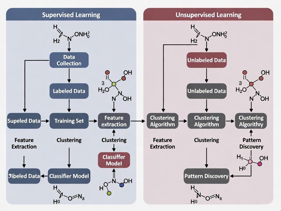
The following diagram illustrates the typical workflows for both approaches, highlighting their distinct processes from data collection to final output.

Comparative Performance Analysis

Empirical studies across diverse species consistently benchmark the performance of these classification methods. The tables below summarize key quantitative findings, providing a reference for researchers to evaluate the expected accuracy and applicability of each technique.

Table 1: Performance of Supervised Learning Methods in Animal Behavior Classification

Species	Behaviors Classified	Supervised Method	Key Predictor Variables	Reported Accuracy	Reference
Thick-billed murres & Black-legged kittiwakes	Standing, swimming, flying, diving	Multiple methods (e.g., threshold, k-means, random forests)	Depth, wing beat frequency, pitch, dynamic acceleration	>98% (murres); 89-93% (kittiwakes)	[12]
Otariids (fur seals & sea lions)	Resting, grooming, feeding, travelling	Support Vector Machine (SVM) with polynomial kernel	Tri-axial acceleration + animal feature statistics	>70% (overall); 52-81% (per-behavior, excluding travel)	[11]
Pre-weaned dairy calves	Lying, standing, walking, running, etc.	Machine learning models (validated on ActBeCalf dataset)	3D-accelerometer data (25 Hz) synchronized with video	92% (2-class model); 84% (4-class model)	[15]

Table 2: Performance and Applications of Unsupervised & Data-Driven Methods

Species / Population	Method	Purpose	Key Findings / Output	Reference
Spotted hyenas, meerkats, coatis	Unsupervised analysis of classified behaviors	Identify underlying patterns in behavioral sequences	Discovery of a common principle: longer engagement in a behavior makes a switch less likely ("decreasing hazard function")	[14]
Adult Humans	K-means Clustering, Latent Profile Analysis	Identify multidimensional physical activity behavior profiles from accelerometry	Discovery of data-driven subgroups (profiles) with distinct associations to health outcomes	[13]
Multiple Taxa (BEBE Benchmark)	Deep Neural Networks (DNNs) vs. Classical Methods	Compare classical ML vs. deep learning for behavior classification	DNNs consistently outperformed classical methods across all 9 tested datasets	[9]

The data reveals that supervised methods are highly accurate for classifying specific, pre-defined behaviors, with performance influenced by the model and feature selection [12] [11]. Unsupervised methods excel at discovering novel patterns and profiles that are not defined a priori, revealing everything from common rules governing behavior transitions in mammals [14] to clinically relevant activity profiles in human populations [13]. Recent benchmarks also indicate that deep neural networks consistently outperform classical machine learning models like random forests, particularly when leveraging self-supervised learning on large datasets [9].

Detailed Experimental Protocols

To ensure reproducibility and provide a clear technical roadmap, this section outlines the standard protocols for implementing both supervised and unsupervised learning approaches with accelerometer data.

Protocol for Supervised Learning

The supervised learning pipeline involves a series of methodical steps from data collection to model validation.

• Data Collection & Annotation:

  • Sensor Deployment: Tri-axial accelerometers are deployed on subjects (e.g., via collars on calves [15] or harnesses on seals [11]) at a suitable sampling frequency (typically ≥25 Hz).
  • Ground-Truthing: Simultaneous video recording is conducted to serve as a gold standard for behavior annotation [15] [11].
  • Behavioral Labeling: Using software like the Behavioral Observation Research Interactive Software (BORIS), annotators meticulously label the video footage, synchronizing the timestamps with the accelerometer data to create a labeled dataset [15]. Inter-observer reliability (e.g., Cohen's Kappa) should be calculated to ensure consistency [15].

• Data Preprocessing & Feature Engineering:

  • The raw accelerometer data is segmented into epochs (e.g., 1-second windows) [12].
  • Informative features are extracted from each epoch. Studies indicate that a small number of critical metrics—such as pitch, dynamic acceleration, and wing-beat frequency for birds [12]—can be sufficient for high accuracy, avoiding over-complexity.

• Model Training & Validation:

  • The labeled dataset is split into training and testing sets.
  • A classification algorithm (e.g., SVM, Random Forest, Neural Network) is trained on the training set.
  • Model performance is rigorously evaluated on the held-out test set using metrics like overall accuracy and per-behavior balanced accuracy [15] [12].

Protocol for Unsupervised Learning

The unsupervised learning workflow is more exploratory, focusing on letting the data reveal its own structure.

• Data Collection & Preprocessing:

  • Accelerometer data is collected as in the supervised approach, but without the need for exhaustive manual labeling.
  • Standard preprocessing (filtering, segmentation) is applied, and general features (e.g., average acceleration, variance) may be extracted across the 24-hour cycle [13].

• Model Application & Pattern Discovery:

  • A clustering algorithm such as K-means or a dimensionality reduction technique is applied to the feature data [13] [10].
  • The algorithm groups epochs or individuals based on the similarity of their movement patterns, without reference to behavior labels.

• Profile Interpretation & Validation:

  • Researchers interpret the resulting clusters by examining their characteristic activity patterns (e.g., "highly active throughout the day" vs. "sedentary with evening activity") to define meaningful profiles or phenotypes [13].
  • The validity and relevance of these data-driven profiles are often tested by examining their association with external health or ecological outcomes [14] [13].

The Scientist's Toolkit: Essential Research Reagents and Materials

Successful implementation of accelerometer-based behavior classification requires a suite of methodological "reagents." The following table details essential components and their functions in a typical research pipeline.

Table 3: Essential Research Reagents for Accelerometer-Based Behavior Classification

Tool / Component	Category	Function / Application	Examples / Notes
Tri-axial Accelerometer	Hardware	Measures acceleration in three perpendicular axes (surge, sway, heave), capturing multi-directional movement.	ActiGraph models [16]; Axy-trek [12]; CEFAS G6a+ [11].
Video Recording System	Hardware	Provides ground-truth data for annotating behaviors and synchronizing with sensor data.	High-up cameras for group pens [15]; handheld cameras for focal follows.
Behavioral Annotation Software	Software	Enables efficient and precise manual labeling of behaviors from video for supervised learning.	BORIS (Behavioral Observation Research Interactive Software) [15].
Bio-logger Ethogram Benchmark (BEBE)	Software/Data	A public benchmark of diverse, annotated datasets for developing and comparing classification methods.	Facilitates cross-species method validation [9].
Supervised Classifiers	Algorithm	Predicts pre-defined behavior labels from accelerometer features.	Support Vector Machine (SVM) [11]; Random Forests [12] [9]; Deep Neural Networks (DNNs) [9].
Unsupervised Clustering Algorithms	Algorithm	Identifies hidden patterns, groups, or profiles within accelerometer data without labels.	K-means [13]; Latent Profile Analysis [13].
Self-Supervised Learning Models	Algorithm	A hybrid approach; a model is pre-trained on a large unlabeled dataset, then fine-tuned with a small labeled set.	DNNs pre-trained on human accelerometer data can be fine-tuned for animal behavior classification [9].

In accelerometer-based behavioral classification, the choice between supervised and unsupervised machine learning is foundational. Supervised learning relies on labeled datasets to train models for predicting known, pre-defined behaviors, while unsupervised learning discovers hidden patterns and structures without labeled training data [17] [18]. This guide objectively compares their performance, with a focused analysis on scenarios where pre-defined behavioral categories make supervised learning the preferred methodology.

Performance and Accuracy Comparison

Empirical studies consistently demonstrate that supervised learning models achieve higher classification accuracy for pre-defined behaviors compared to unsupervised approaches.

The table below summarizes key performance metrics from controlled experiments:

Study Context	Supervised Model & Accuracy	Unsupervised Model & Accuracy	Key Finding
California Condor Behavior [19]	Random Forest (RF): >0.81 overall accuracy, High Kappa [19]	K-means/EM Clustering: <0.8 accuracy, Very low Kappa (0.06 to -0.02) [19]	Supervised RF and kNN were most effective; unsupervised clustering performed poorly.
Classifying Aggressive Child-Toy Interactions [20]	AutoML (Supervised): 0.944 F1-Score, 0.945 AUC [20]	Not Tested	Automated supervised approach achieved high performance for specific behavior.
Female Wild Boar Behavior [21]	Random Forest: 94.8% overall accuracy [21]	Not Tested	Specific behaviors like foraging and lateral resting were identified with high accuracy (up to 97%).

Experimental Protocols in Supervised Learning

Robust supervised learning requires meticulous protocol design. The workflow involves data collection, labeling, model training, and rigorous validation [19] [3]. The diagram below illustrates this multi-stage process for classifying pre-defined behaviors from accelerometer data.

Detailed Methodological Components

• Data Collection and Sensor Placement: Researchers deploy tri-axial accelerometers on subjects, configuring sampling rates (e.g., 1 Hz to 20 Hz) based on battery life and behavior dynamics [19] [21]. Device placement is strategic; for example, ear tags for wild boar [21] or patagial tags for condors [19].

• Ground Truth Labeling and Segmentation: Creating a labeled dataset is the most critical step. Continuous accelerometer data is divided into segments, often using change point detection algorithms for variable-time windows that group similar behavioral events [19]. Each segment is then labeled based on synchronized video observation according to a pre-defined ethogram—a catalog of target behaviors [19].

• Feature Engineering and Model Training: Features are extracted from each labeled data segment. These can include static features (e.g., mean, variance) and dynamic properties [21]. The labeled features are used to train a classifier, such as Random Forest or k-Nearest Neighbor (kNN), which learns the mapping between acceleration patterns and specific behaviors [19].

• Validation and Overfitting Prevention: A portion of the labeled data is held back as a test set. The model's performance on this unseen data is the true measure of its accuracy and generalizability [3]. A significant performance drop between training and test sets indicates overfitting, where the model memorizes training data instead of learning generalizable patterns. Robust validation, such as using independent test sets from different individuals, is essential for credible results [3].

The Scientist's Toolkit: Essential Research Reagents

Successful implementation of supervised learning requires specific "research reagents"—tools and materials that enable the reproducible collection and analysis of behavioral data.

Tool/Reagent	Function & Relevance in Supervised Learning
Tri-axial Accelerometer Tag	The primary data collection tool. It measures acceleration in three dimensions (X, Y, Z), providing the raw waveform data used for classification. [19] [21]
Video Recording System	Serves as the source of "ground truth." Synchronized video is essential for manually labeling accelerometer data segments with the correct pre-defined behaviors. [19]
Pre-defined Ethogram	A structured list of the behaviors of interest (e.g., "sitting," "walking," "foraging"). It standardizes the labeling process, ensuring consistency across observers and studies. [19]
Random Forest Algorithm	A powerful, ensemble supervised learning algorithm. It is frequently used for classification tasks due to its high accuracy and ability to handle complex feature relationships. [19] [21]
AutoML Frameworks	Tools like Auto-WEKA automate the process of algorithm selection and hyperparameter tuning, potentially optimizing model performance with less manual effort. [20]

The experimental evidence clearly indicates that a supervised approach is the superior choice for accelerometer-based behavior classification when research objectives involve identifying a specific, pre-defined set of behaviors. Its strength lies in leveraging labeled ground truth data to build highly accurate and interpretable models, as validated by rigorous testing protocols. While unsupervised learning retains value for exploratory analysis, the demand for precise classification of known behavioral states in fields from wildlife ecology to human medicine solidifies the role of supervised learning as the definitive methodology in these scenarios.

The analysis of complex behavioral data, particularly from sources like accelerometers and video-based pose estimation, presents a significant challenge in research and drug development. Traditional supervised learning approaches rely on pre-defined labels and human annotation, which inherently limits their capacity for discovery. In contrast, unsupervised machine learning is revolutionizing this field by allowing subtle patterns and novel behaviors to emerge directly from the data itself without predetermined categories or labels. This paradigm shift is especially valuable for exploratory analysis where researchers may not know all relevant behavioral categories in advance, or when seeking to identify previously uncharacterized behavioral phenotypes that could inform therapeutic development.

This guide objectively compares the performance of unsupervised approaches against traditional methods, providing researchers with evidence-based insights for methodological selection. By examining experimental data across diverse applications—from wearable accelerometry to rodent behavioral analysis—we demonstrate how unsupervised methods uncover biologically meaningful patterns that might otherwise remain obscured by predefined analytical constraints.

Performance Comparison: Quantitative Evidence

Key Advantages of Unsupervised Approaches

Table 1: Comparative Performance of Unsupervised vs. Traditional Methods

Application Domain	Unsupervised Method	Traditional Method	Performance Metric	Unsupervised Result	Traditional Result
Physical Activity Monitoring in Children [22] [23]	Hidden Semi-Markov Model	Cut-points Thresholding	Correlation with Mobility (R²)	0.51	0.39
Physical Activity Monitoring in Children [22] [23]	Hidden Semi-Markov Model	Cut-points Thresholding	Correlation with Social-Cognitive Capacity (R²)	0.32	0.20
Physical Activity Monitoring in Children [22] [23]	Hidden Semi-Markov Model	Cut-points Thresholding	Correlation with Responsibility (R²)	0.21	0.13
Physical Activity Monitoring in Children [22] [23]	Hidden Semi-Markov Model	Cut-points Thresholding	Correlation with Daily Activity (R²)	0.35	0.24
Human Activity Recognition [24]	Self-Supervised Learning (Pre-trained)	Random Forest	Median Relative F1 Improvement	24.4%	Baseline
Human Activity Recognition [24]	Self-Supervised Learning (Pre-trained)	Deep Learning (From Scratch)	Median Relative F1 Improvement	18.4%	Baseline
Behavior Change Detection [25]	U-BEHAVED Algorithm	N/A (Detection Rate)	Users with Low Variability	80% (400 steps)	N/A
Behavior Change Detection [25]	U-BEHAVED Algorithm	N/A (Detection Rate)	Users with High Variability	80% (1600 steps)	N/A

Limitations and Considerations

While unsupervised approaches demonstrate superior performance in many scenarios, researchers must consider their limitations. Unsupervised models can develop "Clever Hans" effects, where accurate predictions arise from spurious correlations in the data rather than genuine behavioral signals [26]. For example, representation learning models have been shown to rely on text annotations in medical images or background features rather than clinically relevant patterns, which can lead to significant performance degradation under operational conditions [26]. This underscores the importance of applying explainable AI techniques to validate that identified features are biologically or clinically meaningful.

Experimental Protocols and Methodologies

Protocol 1: Unsupervised Physical Activity Analysis with Hidden Semi-Markov Models

Objective: To quantify physical activity intensity from accelerometer data in a diverse pediatric population without relying on population-specific calibration [22] [23].

Equipment: ActiGraph GT3X+ accelerometer, flexible waist-worn belt, Paediatric Evaluation of Disability Inventory-Computer Adaptive Test (PEDI-CAT).

Participant Preparation:

• Fit device snugly around the waist at the mid-axillary line
• Wear for 7 consecutive days during waking hours
• Remove only for bathing, showering, swimming, or sleeping

Data Collection Parameters:

• Sampling frequency: 100 Hz
• Record all movement lasting ≥1 second
• Set device to record two days after parent receives pack

Analytical Procedure:

• Data Segmentation: Divide continuous accelerometer data into discrete segments using a hidden semi-Markov model (HSMM)
• Clustering: Group segments based on movement intensity and patterns without predefined thresholds
• Validation: Compare resulting activity clusters with PEDI-CAT measures of mobility, social-cognitive capacity, responsibility, and daily activity
• Benchmarking: Compare results with traditional cut-points method using thresholds from literature

Key Advantage: This approach allows activity intensity categories to emerge from the data itself rather than imposing external thresholds, making it particularly suitable for diverse or rapidly changing populations where traditional calibration is challenging [22] [23].

Protocol 2: Self-Supervised Learning for Human Activity Recognition

Objective: To leverage large-scale unlabeled accelerometer data (700,000 person-days) to build foundation models that generalize across devices, populations, and environments [24].

Data Preprocessing:

• Utilize UK Biobank accelerometer dataset from ~100,000 participants
• Process 700,000 person-days of free-living, 24/7 human motion data
• Apply multi-task self-supervision with three pretext tasks: arrow of time, permutation, and time warping

Model Architecture:

• Implement deep convolutional neural network for pre-training
• Use weighted sampling to improve convergence across pretext tasks

Training Procedure:

• Pre-training: Train network on unlabeled data using multi-task self-supervision
• Fine-tuning: Adapt pre-trained model to specific downstream activity recognition tasks
• Evaluation: Test on eight benchmark datasets with varying sizes and characteristics

Validation Metrics:

• F1 score and Kappa score across multiple datasets
• Performance in transfer learning scenarios
• Cluster analysis using UMAP for visualization

Key Finding: Self-supervised pre-training consistently improved downstream human activity recognition, especially in small datasets, reducing the need for labeled data while maintaining strong generalization across external datasets [24].

Protocol 3: Early Detection of Physical Activity Behavior Changes

Objective: To detect significant changes in physical activity behavior as they emerge and determine if they become sustained habits [25].

Data Source: Wearable accelerometer step data from 79 users (N=12,798 records).

Algorithm Implementation (U-BEHAVED):

• Streaming Analysis: Periodically scan step data streamed from activity trackers
• Rolling Windows: Compare current behaviors with recent previous ones using rolling time windows
• Change Detection: Identify statistically significant changes in activity patterns
• Habit Classification: Flag new behaviors as potential habits if sustained over time

Validation Approach:

• Test detection rate for behavior changes of varying magnitudes (400-1600 steps)
• Evaluate in users with both low and high variability in physical activity
• Validate habit detection with minimum thresholds of 500-1600 steps per hour

Performance Outcome: The algorithm detected 80% of behavior changes, with step thresholds adapting to individual variability patterns [25].

Research Reagent Solutions

Table 2: Essential Tools for Unsupervised Behavioral Analysis

Tool Category	Specific Solution	Function/Application	Key Features
Accelerometers	ActiGraph GT3X+ [22] [23]	Raw movement data collection	100 Hz sampling, waist-worn, research-grade
Pose Estimation	DeepLabCut [27] [28]	Markerless body movement tracking	Deep learning-based, open-source
Pose Estimation	SLEAP [27]	Animal body part tracking	Multi-animal tracking capability
Behavior Classification	B-SOiD [27]	Unsupervised behavior identification	Open-source, Python-based
Behavior Classification	VAME [27]	Behavioral motif discovery	Variational autoencoder framework
Behavior Classification	Keypoint-MoSeq [27] [28]	Sequencing behavioral motifs	Hidden Markov model approach
Analysis Frameworks	U-BEHAVED [25]	Behavior change detection	Real-time monitoring, habit identification
Analysis Frameworks	Hidden Semi-Markov Models [22] [23]	Activity intensity clustering	Data-driven category emergence

Decision Framework and Implementation

When to Choose an Unsupervised Approach

Optimal Scenarios for Unsupervised Learning:

• Exploratory Research: When investigating new behavioral phenotypes without predefined categories
• Diverse Populations: When studying populations where traditional calibration fails (e.g., children with diverse developmental abilities [22] [23])
• Novel Behavior Discovery: When seeking to identify previously uncharacterized behavioral patterns or sequences
• Large Unlabeled Datasets: When leveraging massive datasets where manual labeling is impractical (e.g., 700,000 person-days of accelerometer data [24])
• Individualized Assessment: When behavior change detection needs to be personalized to individual baseline patterns [25]

Scenarios Where Supervised Approaches May Be Preferable:

• Well-Established Behavioral Categories: When studying previously validated behavioral classifications with sufficient labeled data
• Specific Hypothesis Testing: When investigating predefined behavioral outcomes rather than exploring novel patterns
• Limited Computational Resources: When unsupervised model validation and interpretation is not feasible

Implementation Workflow

The following diagram illustrates a typical workflow for implementing unsupervised behavior analysis:

Figure 1: Unsupervised Behavior Discovery Workflow

U-BEHAVED Algorithm Process

The U-BEHAVED algorithm for detecting physical activity behavior changes follows this specific process:

Figure 2: U-BEHAVED Behavior Change Detection Process

Unsupervised approaches offer transformative potential for exploratory analysis and novel behavior discovery in accelerometer data and beyond. The experimental evidence demonstrates their superiority in diverse populations, their ability to detect subtle behavior changes, and their capacity to identify meaningful patterns without predefined labels. While requiring careful validation to avoid spurious correlations, these methods enable researchers to move beyond known behavioral categories and discover genuinely novel phenotypes—a crucial capability for advancing both basic research and therapeutic development.

Researchers should consider adopting unsupervised approaches when working with diverse populations where traditional methods fail, when exploring new behavioral domains without established categories, or when leveraging large-scale unlabeled datasets. The continued development of explainable AI techniques will further enhance our ability to validate and interpret discoveries made through these powerful unsupervised methods.

Comparative Strengths and Weaknesses at a Glance

The analysis of accelerometer data for behavior classification is a cornerstone of modern movement ecology, biomedical research, and drug development. The selection between supervised and unsupervised machine learning approaches represents a fundamental methodological decision that directly impacts research outcomes, interpretation, and validity. Supervised learning relies on labeled datasets where accelerometer data is paired with directly observed behaviors, enabling the training of models to predict known behavioral categories [3] [29]. In contrast, unsupervised learning identifies inherent patterns and structures within accelerometer data without pre-existing labels, potentially revealing previously unclassified behaviors [1] [29]. This guide provides a systematic comparison of these approaches, synthesizing experimental data and methodologies to inform researchers' analytical decisions.

Comparative Analysis of Classification Approaches

Table 1: High-level comparison of supervised and unsupervised classification approaches

Feature	Supervised Learning	Unsupervised Learning
Data Requirements	Requires labeled training data with observed behaviors [3]	No labeled data needed; works with raw accelerometer data [1] [29]
Primary Output	Classification into predefined behavioral categories [3] [29]	Identification of behavioral clusters based on signal similarity [1]
Implementation Complexity	High (feature engineering, model training, validation) [3] [30]	Moderate (cluster identification and interpretation) [1]
Validation Approach	Performance metrics on test sets (accuracy, precision, recall) [3] [29]	Manual labeling of clusters for validation [1]
Key Strengths	Predicts known behaviors directly; higher agreement with ground truth [1]	Discovers novel behaviors; no need for extensive labeling [1] [29]
Key Limitations	Vulnerable to overfitting; dependent on labeled data quality [3]	Clusters may not align with biologically meaningful behaviors [1]

Table 2: Experimental performance comparison across studies

Study Context	Supervised Performance	Unsupervised Performance	Agreement Between Approaches
Penguin Behavior Classification [1]	Random Forest: >80% agreement with unsupervised	Expectation Maximization: 12 behavioral classes identified	>80% overall, with outliers <70% for behaviors with signal similarity
Animal Behavior Classification [29]	SVM, ANN, RF, XGBoost performed well with proper validation	k-means clustering applied but requires manual interpretation	Not directly quantified
Human Activity Recognition [31]	Hybrid DeepF-SVM: 93.57-98.48% accuracy on benchmark datasets	Not evaluated	Not applicable
Wild Red Deer Behavior [4]	Discriminant Analysis: Accurate multiclass classification	Not the focus of study	Not applicable

Detailed Methodological Protocols

Supervised Learning Workflow

Supervised learning for accelerometer behavior classification follows a structured pipeline. First, researchers collect raw accelerometer data while simultaneously conducting behavioral observations to create labeled datasets [4]. The data is then segmented into windows, typically ranging from 6-second non-overlapping windows in human studies [30] to 5-minute intervals in wildlife research [4]. Feature extraction follows, calculating time-domain features (mean, standard deviation, skewness) and frequency-domain features (spectral entropy, frequency bands) from the raw signals [30] [31]. The labeled dataset is split into training (typically 70%) and testing (30%) subsets [30] [4]. Model selection and training proceed using algorithms such as Random Forest, Support Vector Machines, or Artificial Neural Networks [30] [29]. Critical validation through independent test sets assesses performance metrics including accuracy, precision, recall, and F1-score [3] [29]. Finally, the trained model deploys to classify new, unlabeled accelerometer data [29].

Unsupervised Learning Workflow

The unsupervised learning methodology begins with raw accelerometer data collection without behavioral labels [1]. Data undergoes similar preprocessing and segmentation as in supervised approaches. Feature calculation generates relevant input variables for clustering algorithms [1]. Cluster analysis applies algorithms such as Expectation Maximization or k-means to identify natural groupings within the data [1] [29]. Researchers then manually interpret these clusters by examining characteristic signal patterns and, when possible, correlating with limited behavioral observations [1]. The identified behavioral classes validate through comparison with independent datasets or expert assessment [1]. For enhanced utility, unsupervised outputs sometimes train supervised models, creating a hybrid approach that leverages the strengths of both methods [1].

Performance and Validation Considerations

Overfitting Risks in Supervised Learning

A critical challenge in supervised learning is overfitting, where models perform well on training data but fail to generalize to new datasets [3]. A systematic review of 119 accelerometer-based behavior classification studies revealed that 79% (94 papers) did not adequately validate their models to robustly identify potential overfitting [3]. Overfitting occurs when model complexity approaches or surpasses data complexity, causing the model to memorize training instances rather than learning generalizable patterns [3]. Detection requires rigorous validation using independent test sets completely unseen during training [3]. Common practices that mask overfitting include non-independent test sets, non-representative test set selection, failure to tune hyperparameters on validation sets, and optimization on inappropriate performance metrics [3].

Agreement Between Approaches

Research comparing supervised and unsupervised methods reveals generally high agreement. In penguin behavior classification, integrated unsupervised and supervised approaches demonstrated greater than 80% agreement in behavioral classifications, with minimal differences in energy expenditure estimates [1]. However, outliers with less than 70% agreement occurred for behaviors characterized by signal similarity, highlighting challenges in distinguishing mechanically similar activities [1]. This suggests that while both approaches generally converge, certain behaviors remain challenging regardless of methodology.

Computational Performance for On-Board Classification

For applications requiring real-time classification on resource-constrained devices, computational efficiency becomes critical. Studies evaluating machine learning classifiers for next-generation smart trackers identified Random Forest (RF), Artificial Neural Networks (ANN), and Extreme Gradient Boosting (XGBoost) as suitable for on-board classification due to favorable runtime and storage requirements [29]. These algorithms maintained performance even with reduced feature sets, minimizing computational demands while preserving classification accuracy [29].

Essential Research Reagents and Tools

Table 3: Essential research toolkit for accelerometer-based behavior classification

Tool Category	Specific Examples	Function and Application
Accelerometer Sensors	Tri-axial accelerometers [4] [32]; 9-axis IMUs (accelerometer, gyroscope, magnetometer) [33]	Capture raw movement data on multiple axes; IMUs provide complementary orientation information
Data Processing Tools	SENS motion software [32]; ActiPASS [32]; Custom MATLAB/Python scripts	Preprocess raw data, extract features, and implement classification algorithms
Supervised Algorithms	Random Forest [4] [1] [29]; SVM [30] [29] [31]; CNN [34] [31]; Artificial Neural Networks [30] [29]	Classify behaviors from labeled training data; range from traditional ML to deep learning approaches
Unsupervised Algorithms	Expectation Maximization [1]; k-means clustering [29]	Identify natural groupings in unlabeled accelerometer data
Validation Methods	Independent test sets [3]; Cross-validation [3]; Manual cluster interpretation [1]	Assess model generalizability and prevent overfitting
Performance Metrics	Accuracy, Precision, Recall, F1-score [34] [31]; Cohen's Kappa [32]; Balanced Accuracy [32]	Quantify classification performance and model effectiveness

The selection between supervised and unsupervised approaches for accelerometer-based behavior classification involves fundamental trade-offs between methodological rigor, data requirements, and interpretability. Supervised learning provides direct classification into predefined behavioral categories with higher agreement to ground truth but requires extensive labeled data and risks overfitting without proper validation [3] [1]. Unsupervised learning discovers novel behaviors without labeling effort but produces clusters that may not align with biologically meaningful categories [1] [29]. Emerging hybrid approaches that combine unsupervised cluster identification with subsequent supervised classification leverage the strengths of both methods [1]. The choice ultimately depends on research objectives, data availability, and computational resources, with both approaches offering distinct advantages for advancing behavioral research in ecological, biomedical, and pharmaceutical contexts.

From Data to Discovery: Methodological Workflows and Real-World Applications

The fundamental difference between supervised and unsupervised learning paradigms in accelerometer-based behavior classification is the reliance on labeled data. Supervised learning requires a ground-truthed dataset where acceleration signals are paired with corresponding behavior labels (e.g., foraging, resting, walking) [21] [4]. This labeled dataset serves as the foundational teacher, enabling models to learn patterns that distinguish different behaviors. In contrast, unsupervised approaches identify inherent patterns or clusters in accelerometer data without predefined labels, making them suitable for exploratory analysis but less effective for precise behavior identification [35] [36]. The quality, volume, and methodological rigor applied during data labeling and validation directly dictate the performance and reliability of the resulting classification models [37] [3].

This comparison guide examines the complete supervised learning pipeline for accelerometer data, focusing on experimental evidence that quantifies performance differences between methodological approaches. We present structured comparisons of annotation strategies, sensor configurations, algorithm performance, and validation protocols to equip researchers with evidence-based guidance for developing robust behavioral classification systems.

Data Labeling Strategies: Balancing Quality, Speed, and Cost

The initial phase of the supervised learning pipeline involves creating high-quality labeled datasets through various annotation strategies, each offering distinct trade-offs between quality, control, scalability, and cost [37] [35].

Table: Comparison of Data Labeling Approaches for Behavioral Research

Approach	Key Advantages	Key Limitations	Best Suited For
In-House Labeling	High control, domain expertise utilization, data privacy [38] [36]	Expensive, time-consuming, management overhead [38] [36]	Projects with sensitive data or requiring specialized expertise [38]
Crowdsourcing	Cost-effective, rapid scaling, flexibility [36]	Questionable quality, inconsistent results, limited domain knowledge [38] [36]	Non-specialized tasks with limited budgets and flexible quality requirements [38]
Third-Party Partners	High quality, technical expertise, cost-efficient at scale [38]	Relinquished control, can be expensive [38]	Large-scale projects requiring high-quality labels and technical guidance [38]
Programmatic/Semi-Supervised	Rapid scaling, combines human expertise with automation [37] [35]	Potential quality issues, requires technical setup [35]	Large datasets where manual labeling is impractical [37] [35]

Each strategy represents a different point on the spectrum of the data labeling trade-off. For specialized behavioral research, a hybrid approach often yields optimal results. For instance, subject matter experts can establish a ground-truth dataset and develop labeling guidelines, while automated methods or crowdsourced workers handle initial annotations, with expert review reserved for edge cases or quality assurance [37].

Experimental Comparisons: Sensor Configurations and Algorithm Performance

Sensor Fusion Enhances Classification Accuracy

Experimental evidence demonstrates that combining multiple sensor modalities significantly improves classification performance over single-sensor approaches. A comprehensive study on dairy cow behavior classification collected over 780,000 labeled observations to compare accelerometer-only, gyroscope-only, and combined sensor models [39].

Table: Performance Comparison of Sensor Configurations for Cattle Behavior Classification

Behavior	Accelerometer-Only Model	Gyroscope-Only Model	Combined Sensor Model
Lying	High accuracy	High accuracy	Consistently superior performance
Standing	Moderate accuracy	Moderate accuracy	Consistently superior performance
Eating	High variability	High rotational activity capture	Improved robustness across individuals
Walking	Lower sensitivity	Better rotational detection	Improved classification robustness

The integration of accelerometer and gyroscope data was particularly valuable for distinguishing behaviors with similar postures but different movement characteristics, such as standing versus eating. Gyroscope sensors (GyroY and GyroZ axes) captured the highest rotational activity during eating and walking behaviors, providing complementary information to the linear acceleration data [39].

Algorithm Selection Significantly Impacts Model Performance

Comparative studies across multiple species reveal substantial performance differences between machine learning algorithms, influenced by data characteristics, preprocessing methods, and behavioral complexity. Research on wild red deer compared multiple algorithms using minmax-normalized acceleration data from multiple axes and their ratios [4] [40].

Discriminant analysis generated the most accurate classification models, successfully differentiating between lying, feeding, standing, walking, and running behaviors in alpine environments [4]. The study highlighted that algorithm performance varied significantly depending on the transformation method and combination of input variables used.

In human movement studies comparing deep learning (DL) and classical machine learning approaches for classifying 24-hour movement behaviors from wrist-worn accelerometers, Long Short-Term Memory (LSTM) networks achieved approximately 85% overall accuracy when trained on raw acceleration signals [41]. Classical algorithms including Random Forest, when trained on handcrafted features, achieved overall accuracy ranging from 70% to 81%, with higher confusion observed between moderate-to-vigorous physical activity and light physical activity categories compared to sleep and sedentary behaviors [41].

Sampling Strategies and Data Resolution Trade-Offs

The trade-off between data resolution and practical constraints like battery life presents significant methodological considerations for long-term behavioral studies. Research on wild boar demonstrated that low-frequency accelerometers (1 Hz) can successfully classify behaviors including foraging, lateral resting, sternal resting, and lactating with accuracies ranging from 50% (walking) to 97% (lateral resting) using random forest models [21].

This approach addresses critical constraints in wildlife research where frequent recapture for battery replacement causes severe stress and potential mortality [21]. Low-frequency sampling enables extended monitoring periods essential for capturing seasonal and inter-annual behavioral trends, despite some limitation in classifying dynamic behaviors like walking.

Methodological Protocols: Experimental Workflows for Behavioral Classification

Standardized Data Collection and Annotation Protocols

Robust behavioral classification requires meticulous experimental design and data collection protocols. The red deer study implemented a comprehensive methodology where animals were fitted with GPS collars containing accelerometers measuring movement on multiple axes at 4 Hz, with data averaged over 5-minute intervals [4]. The key innovation was collecting simultaneous behavioral observations in wild environments, creating labeled datasets where acceleration data served as input variables and observed behaviors as output variables [4].

The dairy cow study employed even more rigorous annotation protocols, using two trained observers who independently annotated behaviors from synchronized video recordings across a 90-day period [39]. Inter-observer reliability was quantified using Cohen's Kappa (κ=0.84), with discrepancies resolved through discussion and consensus meetings. This approach ensured high-quality ground truth labels for model training and evaluation [39].

Validation Practices to Prevent Overfitting

A systematic review of 119 studies using accelerometer-based supervised learning revealed critical gaps in validation practices, with 79% of studies not adequately validating their models to detect overfitting [3]. Overfitting occurs when models memorize specific instances in training data rather than learning generalizable patterns, leading to poor performance on new data [3].

Recommended validation practices include:

• Independent test sets: Completely separate from training data
• Individual-level splitting: When classifying behavior across multiple subjects, splitting data by individual rather than randomly pooling all data points
• Appropriate performance metrics: Using metrics that account for class imbalance common in behavioral datasets
• Cross-validation: Employing k-fold or leave-one-subject-out cross-validation where appropriate

The red deer study addressed class imbalance by developing a novel performance metric that accounted for unequal behavior distribution, providing a more realistic assessment of model utility [4].

The Scientist's Toolkit: Essential Research Reagents and Solutions

Table: Essential Research Toolkit for Accelerometer-Based Behavioral Classification

Tool/Resource	Function/Purpose	Examples/Alternatives
Tri-axial Accelerometers	Measures linear acceleration in three dimensions (X, Y, Z axes)	Commercial wildlife collars (VECTRONIC), research-grade sensors (Axivity AX3) [4] [41]
Gyroscope Sensors	Captures angular velocity and rotational movements	MPU-6050 sensors used in cattle study [39]
Data Annotation Platforms	Tools for creating labeled behavioral datasets	Label Studio, Prodigy, Amazon SageMaker Ground Truth [37]
Machine Learning Environments	Programming environments for model development	R with h2o package, Python with scikit-learn, TensorFlow, PyTorch [21] [39]
Validation Frameworks	Methods to assess model generalizability and detect overfitting	Cross-validation, independent test sets, performance metrics for imbalanced data [3] [4]

Experimental evidence consistently demonstrates that supervised learning approaches using high-quality labeled datasets achieve superior precision in classifying specific behaviors compared to unsupervised methods. Key findings from comparative studies indicate:

• Sensor fusion of accelerometer and gyroscope data consistently outperforms single-sensor approaches, particularly for distinguishing behaviors with similar postures but different movement patterns [39]
• Algorithm selection significantly impacts performance, with discriminant analysis excelling in wild red deer classification [4] and Random Forest with sensor fusion achieving high accuracy in cattle monitoring [39]
• Low-frequency sampling (1 Hz) can successfully classify many behaviors while enabling long-term battery life essential for wildlife studies [21]
• Rigorous validation using independent test sets is critical but frequently overlooked, with 79% of reviewed studies insufficiently validating for overfitting [3]

For researchers designing behavioral classification studies, we recommend: investing in high-quality data labeling with expert annotation where possible; implementing sensor fusion approaches when monitoring complex behaviors; selecting algorithms based on empirical comparison rather than default preferences; and employing rigorous validation protocols with completely independent test sets. These practices ensure developed models will generalize effectively to new individuals and environmental conditions, advancing the reliability and applicability of accelerometer-based behavioral classification across research domains.

Unsupervised machine learning, particularly clustering, serves as a powerful approach for identifying inherent patterns in complex datasets without prior knowledge of outcomes. This capability is especially valuable in fields like behavioral analysis using accelerometer data, where labeled data is scarce and populations are diverse. This guide provides a comparative analysis of unsupervised clustering methodologies against supervised alternatives, detailing performance metrics, experimental protocols, and practical implementation workflows to inform researchers and development professionals in selecting appropriate techniques for their specific applications.

Machine learning classification strategies are broadly categorized into supervised and unsupervised paradigms. Supervised learning requires a labeled dataset to train models for predicting known outcomes, while unsupervised learning seeks to identify the inherent structure of unlabeled data to discover novel patterns or natural groupings [42]. Clustering, a cornerstone of unsupervised learning, is increasingly critical for analyzing complex data from sources like wearable accelerometers, where manual labeling is impractical and the underlying categories may not be fully known [19] [22]. The core strength of clustering lies in its data-driven approach, which can reveal meaningful subgroups within heterogeneous populations—such as distinct physical activity states in children [22] or patient phenotypes in heart failure cohorts [43]—without the constraints and potential biases of pre-defined labels. This guide systematically compares the performance of various clustering techniques against supervised and semi-supervised alternatives, providing a foundation for methodological selection in research and development.

Comparative Performance: Unsupervised vs. Supervised and Semi-Supervised Methods

The effectiveness of learning algorithms varies significantly depending on the data characteristics and analytical goals. The table below summarizes a comparative study on classifying behaviors from accelerometer data in California condors, illustrating a typical performance hierarchy.

Table 1: Classification Performance Across Machine Learning Approaches (California Condor Accelerometer Data) [19]

Learning Type	Specific Algorithms	Overall Accuracy	Kappa Statistic	Notes
Unsupervised	K-means, EM Clustering	< 0.8	-0.02 to 0.06	Poor performance, very low Kappa
Semi-Supervised	Nearest Mean Classifier	0.61	N/A	Effective for only 2 of 4 behavior classes
Supervised	Random Forest (RF), k-Nearest Neighbor (kNN)	> 0.81	Highest	Most effective across all behavior types

This case study demonstrates a common finding: while unsupervised methods are valuable for exploration, supervised models often achieve higher accuracy for well-defined classification tasks where labeled training data is available [19] [42]. However, this performance gap narrows or reverses in scenarios where labels are unavailable, costly to produce, or when the objective is to discover new, previously undefined categories.

Experimental Protocols in Unsupervised Accelerometer Research

To ensure reproducible and valid results, studies employing unsupervised learning for accelerometer data follow rigorous experimental protocols. The following workflow generalizes the common steps, from data collection to cluster interpretation.

Diagram 1: Experimental Workflow for Unsupervised Accelerometer Analysis

Data Collection and Preprocessing

Data is typically collected from wearable, tri-axial accelerometers set to record at frequencies between 20-100 Hz [19] [22]. Preprocessing is critical and involves:

• Segmentation: Dividing continuous data into analyzable units. Variable-time segmentation, which uses change points in the data to define boundaries, often improves classification accuracy by grouping similar behaviors [19].
• Feature Extraction: Calculating summary metrics from raw acceleration signals. Common features in the literature include mean, standard deviation, skewness, kurtosis, and dominant frequency [44].

Feature Selection and Dimensionality Reduction

Given the high dimensionality of feature-extracted accelerometer data, feature selection and dimensionality reduction are essential to avoid the "curse of dimensionality" and prevent model overfitting [45] [44]. The most prevalent technique identified in a systematic review is Principal Component Analysis (PCA), which projects original features into a new, lower-dimensional space while retaining maximum information [44]. Correlation matrices are also frequently used to select a subset of features that are highly correlated with cluster membership but uncorrelated with each other [44].

Clustering Algorithm Application and Validation

The core of the pipeline is applying clustering algorithms to the processed data. A benchmark study on univariate data recommends testing multiple algorithms, as performance is highly dependent on the data type [45]. Key steps include:

• Algorithm Selection: Common choices include partitioning methods like K-means and Partitioning Around Medoids (PAM), density-based methods like DBSCAN, and neural models like Self-Organizing Maps [43] [44] [46].
• Cluster Number (NoC) Estimation: The optimal number of clusters is determined using internal validation indices. A robust approach involves using a histogram of predictions from multiple indices (e.g., silhouette width, Dunn Index) to estimate the final NoC [43] [45].
• Validation: Internal validation indices assess the compactness and separation of the resulting clusters. For example, the PAM algorithm was validated as superior in an HFpEF patient study because it produced six distinct, clinically meaningful clusters with statistically different outcomes, whereas hierarchical clustering yielded groups that were too small, and K-prototype showed significant overlap [43].

Performance Benchmarking of Clustering Algorithms

Direct benchmarking of algorithms on datasets with known classes provides the most reliable guidance for selection. The following table synthesizes findings from a large-scale benchmark study on univariate data and a clinical study on patient phenotyping.

Table 2: Benchmarking of Unsupervised Clustering Algorithms [43] [45]

Clustering Algorithm	Classification	Key Findings & Performance Notes
Partitioning Around Medoids (PAM)	Partitioning	Superior group separation in clinical data; robust to noise. Identified 6 distinct HFpEF phenotypes with different mortality [43].
K-means / K-prototype	Partitioning	Commonly used but may show significant overlap between clusters. Performance is highly dependent on feature space construction [43] [45].
Hierarchical Clustering	Hierarchical	May produce too many small, clinically meaningless clusters. Generated clusters with only 2 and 7 members in a patient cohort [43].
Fuzzy C-means (FCM)	Fuzzy	Included in top performers for univariate data benchmarking [45].
Gustafson-Kessel (GK)	Fuzzy	Included in top performers for univariate data benchmarking [45].
DBSCAN	Density-Based	Does not require pre-specification of cluster number; can identify noise points [44].

The benchmark study on simulated nanoelectronics data concluded that careful selection of both the feature space construction method and the clustering algorithm is critical, as their interaction can greatly impact classification accuracy [45].

Case Study: Hidden Semi-Markov Model (HSMM) vs. Cut-Points for Physical Activity

A compelling application of unsupervised learning is using accelerometer data to quantify physical activity in children, a rapidly changing and diverse population.

Experimental Protocol

In a study with 279 children aged 9-36 months, a Hidden Semi-Markov Model (HSMM) was applied to waist-worn ActiGraph accelerometer data [22]. The HSMM is a data-driven approach that segments and clusters the accelerometer trace without relying on pre-calibrated thresholds, allowing activity intensity states to emerge from the data itself [22]. This was compared directly to the traditional cut-points approach, which classifies activity intensity based on thresholds calibrated against energy expenditure in a lab setting [22] [47].

Performance and Clinical Relevance

The unsupervised HSMM approach demonstrated a stronger correlation with the children's developmental abilities, as measured by the Paediatric Evaluation of Disability Inventory (PEDI-CAT).

Table 3: Correlation with Developmental Abilities (R²): HSMM vs. Cut-Points [22]

PEDI-CAT Domain	HSMM (Unsupervised)	Cut-Points (Traditional)
Mobility	0.51	0.39
Social-Cognitive	0.32	0.20
Responsibility	0.21	0.13
Daily Activities	0.35	0.24
Age	0.15	0.10

The results show that the HSMM consistently explained more variance in developmental scores, establishing it as a more sensitive and appropriate method for quantifying physical activity in heterogeneous or rapidly changing populations [22]. This case highlights a key advantage of unsupervised methods: they do not require costly calibration studies and can generalize better across diverse populations.

The Scientist's Toolkit: Essential Research Reagents and Materials

The following table catalogues key computational tools and materials referenced in the featured experiments for replicating unsupervised clustering studies.

Table 4: Research Reagent Solutions for Unsupervised Accelerometer Analysis

Reagent / Solution	Function / Purpose	Example Use Case
ActiGraph GT3X+	A research-grade accelerometer for collecting raw tri-axial acceleration data.	Primary data collection device in the Hidden Semi-Markov Model (HSMM) study of children's physical activity [22].
GENEActiv	A wrist-worn, raw-data accelerometer with a wide dynamic range (±8g).	Used to capture accelerometer data in the Millennium Cohort Study at age 14 [47].
R Package 'GGIR'	An open-source software for processing raw accelerometer data, including calibration, non-wear detection, and metric extraction.	Used to preprocess raw acceleration data into vector magnitude (ENMO) and orientation angles [47].
Gower Distance Metric	A similarity measure that handles mixed data types (numeric and categorical) by scaling results between 0 and 1.	Used by the PAM algorithm in the HFpEF patient clustering study, contributing to its superior performance [43].
t-SNE (t-distributed SNE)	A non-linear dimensionality reduction technique ideal for visualizing high-dimensional data in 2D or 3D.	Employed for visualizing high-dimensional cluster outcomes in the HFpEF study [43] and benchmarked in [45].
Silhouette Width Index	An internal cluster validation index that measures how similar an object is to its own cluster compared to other clusters.	Used to determine the optimal number of clusters by evaluating compactness and separation [43].

The choice between supervised and unsupervised learning for classification is context-dependent. Supervised methods like Random Forest excel in accuracy when classifying data into known, well-defined categories with sufficient labeled examples [19]. However, unsupervised clustering is an indispensable tool for exploratory data analysis, patient or behavior phenotyping, and studies of diverse populations where labeled data is a barrier. As evidenced by the superior clinical correlation of HSMM in quantifying children's physical activity, unsupervised methods can provide more sensitive and appropriate solutions for real-world, heterogeneous data [22]. A robust analytical strategy involves benchmarking multiple clustering algorithms and feature space constructions specific to the measurement type to achieve optimal performance [45].

Feature Engineering and Selection for Robust Classification

The expanding field of movement ecology, human health monitoring, and industrial predictive maintenance increasingly relies on data from accelerometers. A critical challenge in translating raw sensor data into meaningful classifications—whether of animal behavior, human activities, or machine faults—lies in the processes of feature engineering and selection. These steps are paramount for building robust, generalizable machine learning models, especially within a research paradigm that compares the efficacy of supervised versus unsupervised learning approaches. Supervised learning, which relies on labeled datasets to train models, remains the dominant method for behavior classification from accelerometer data [3] [9]. However, its performance is highly contingent on the features used to represent the underlying signal. This guide objectively compares the performance of different feature engineering and selection methodologies, providing researchers with the experimental data and protocols needed to inform their own analytical workflows.

Comparative Performance of Feature Engineering and Selection Methods

The choice of how to process, engineer, and select features from raw accelerometer data significantly impacts the performance and generalizability of classification models. The following tables summarize quantitative results from recent studies across biological and engineering domains.

Table 1: Performance Comparison of Feature Engineering and Selection Methods in Ecological Studies

Study & Species	Feature Engineering Approach	Selection/Method	Classification Model	Key Performance Metric & Result
Wild Red Deer [4]	Min-max normalization; Ratios of multiple axes	Model-based optimization	Discriminant Analysis	High accuracy for lying, feeding, standing, walking, running
Javan Slow Loris [48]	Hand-crafted features from raw accelerometer data	Not Specified	Random Forest	Resting: 99.16%; Feeding: 94.88%; Locomotion: 85.54%
Multi-Species Benchmark (BEBE) [9]	Deep features from raw data (via CNN/RNN)	Embedded in architecture	Deep Neural Networks	Outperformed classical ML methods across all 9 tested datasets
Multi-Species Benchmark (BEBE) [9]	Hand-crafted summary statistics (features)	Not Specified	Random Forest (Classical ML)	Lower performance than deep neural networks across all datasets

Table 2: Performance in Human Health and Industrial Applications

Study & Application	Feature Engineering Approach	Selection/Method	Classification Model	Key Performance Metric & Result
Smartphone Fall Detection [49] [50]	64 statistical features from 3s windows with two 50% overlapping sub-windows (3s2sub)	Not Specified	K-Nearest Neighbors (KNN)	99.89% accuracy (MobiAct dataset); 98.45% accuracy (UniMiB SHAR, LOSO)
Smartphone Fall Detection [49] [50]	64 statistical features from 3s windows with two 50% overlapping sub-windows (3s2sub)	Not Specified	Support Vector Machine (SVM)	95.35% sensitivity, 98.12% specificity (FARSEEING dataset)
Gearbox Failure [51]	64 time-domain statistical condition indicators (CIs)	Wrapper method with Random Forest	Random Forest (RF)	>98% accuracy and AUC
Gearbox Failure [51]	7 most relevant CIs (selected from 64)	Wrapper method with Random Forest	K-Nearest Neighbors (K-NN)	>98% accuracy and AUC
Dairy Cattle Lameness [52]	Raw accelerometer data	Dimensionality Reduction (PCA/fPCA)	Multiple ML Models	fPCA with fCV gave most robust performance for independent farm data

Detailed Experimental Protocols

To ensure reproducibility and provide a clear framework for future research, this section outlines the detailed methodologies from key cited studies that demonstrated high classification performance.

Wrapper-Based Feature Selection for Gearbox Failure Severity

This methodology [51] provides a structured, automated framework for selecting the most informative time-domain features.

• Data Acquisition: Vibration signals were acquired using six accelerometers (A1–A6) mounted at different positions and inclinations on a spur gearbox test bench. Data was sampled at 50 kHz over a 10-second period, generating 500,000 data points per sensor per run. Four failure types (breaking, cracking, pitting, scuffing) were simulated and tested across nine progressive severity levels.
• Feature Extraction: From the raw vibration signals, 64 statistical condition indicators (CIs) were calculated in the time domain. These included conventional metrics (e.g., root mean square, kurtosis, skewness) and non-conventional ones (e.g., waveform length, Wilson amplitude).
• Feature Selection - Wrapper Method:
  • Phase 1 (Model Optimization and Ranking): A Random Forest (RF) classifier was trained using all 64 CIs from accelerometers A1-A3. The model's hyperparameters were optimized, and the mean influence (MI) of each CI on the model's accuracy was calculated, generating a ranked list.
  • Phase 2 (Cross-Failure Analysis): The top 10 CIs from each accelerometer (A1-A3) were assigned a descending weight (10 for most important, 1 for least). These weights were then summed by failure type.
  • Phase 3 (Aggregation): The weights for each CI were aggregated across all failure types. The seven CIs with the highest total weights were selected as the final, most informative subset for subsequent classification tasks.
• Validation: The selected 7-CI subset was validated using data from the hold-out accelerometers (A4-A6) and achieved >98% accuracy with both RF and K-NN classifiers, demonstrating robustness to sensor placement.

The3s2subFeature Engineering Method for Fall Detection

This protocol [49] details a novel windowing and feature extraction strategy optimized for classifying short-duration events like falls.

• Data Preparation: Raw tri-axial accelerometer data from smartphones is used as input.
• Windowing and Sub-windowing:
  • The data stream is segmented into a 3-second window.
  • This 3-second window is then divided into two overlapping sub-windows, with a 50% overlap ratio.
• Feature Extraction: A comprehensive set of 64 statistical features (e.g., mean, standard deviation, min, max, correlation between axes) is extracted from each of the two sub-windows and from the entire 3-second window.
• Classification: The combined set of features is fed into a classifier, such as K-Nearest Neighbors (KNN) or Support Vector Machine (SVM), to detect a fall event.
• Validation: The method was rigorously evaluated through same-dataset (e.g., Leave-One-Subject-Out on UniMiB SHAR) and, crucially, cross-dataset validation (training on UniMiB SHAR, testing on MobiAct and the real-world FARSEEING dataset), proving its robustness.

Dimensionality Reduction for High-Dimensional Animal Data

This protocol [52] addresses the challenge of "wide" data, where the number of features (accelerometer data points) far exceeds the number of subjects.

• Data Challenge: Accelerometer data from dairy cows was high-dimensional, creating a high risk of overfitting for standard machine learning models.
• Approaches Compared:
  • Raw Data: Applying ML models directly to the accelerometer data.
  • Principal Component Analysis (PCA): Reducing data dimensionality by transforming features into linearly uncorrelated principal components.
  • Functional PCA (fPCA): A specialized technique that accounts for the time-series nature of the data, often preserving more meaningful information than standard PCA.
• Critical Validation Step: The study highlights the importance of validation strategy. It compared:
  • n-Fold Cross-Validation (nCV): Standard random data splitting.
  • Farm-Fold Cross-Validation (fCV): Where data from entire farms are held out as test sets.
• Outcome: The combination of fPCA for feature reduction and farm-fold cross-validation (fCV) for evaluation provided the most realistic and robust estimate of model performance when applied to new, independent farms, significantly outperforming models tested with nCV.

Workflow Visualization

The following diagram illustrates the logical sequence and decision points in a robust feature engineering and classification pipeline, synthesizing the most effective methods from the cited protocols.

Feature Engineering and Selection Workflow

The Scientist's Toolkit

This section catalogs essential reagents, tools, and algorithms that form the foundation of rigorous accelerometer-based classification research.

Table 3: Essential Research Reagents and Solutions for Accelerometer Classification

Item Name	Function/Application	Example/Note
Tri-axial Accelerometer	Measures acceleration in three perpendicular axes (X, Y, Z), capturing posture and dynamic movement.	AX3 Logging 3-axis accelerometer is commonly used in animal [52] and human [53] studies.
Labeled Dataset (Supervised)	Provides ground-truthed data for training and validating supervised ML models.	BEBE benchmark [9], UniMiB SHAR, MobiAct, FARSEEING [49].
Random Forest Classifier	A versatile ensemble learning method that also provides feature importance scores.	Used for behavior classification [48] and as the engine for wrapper-based feature selection [51].
K-Nearest Neighbors (KNN)	A simple, effective classifier for time-series data, often used as a benchmark.	Achieved 99.89% accuracy in fall detection with the 3s2sub method [49].
Principal Component Analysis (PCA)	A classical linear technique for reducing data dimensionality and mitigating overfitting.	Compared against fPCA for dairy cattle lameness detection [52].
Functional PCA (fPCA)	A specialized dimensionality reduction technique that accounts for the time-series structure of data.	Outperformed standard PCA for classifying accelerometer data from dairy cows [52].
Wrapper Method	A feature selection technique that uses the performance of a ML model to evaluate feature subsets.	Effectively identified the 7 most relevant condition indicators from 64 candidates [51].
Cross-Dataset Validation	A rigorous validation protocol that tests a model on data from a different source than its training data.	Critical for proving model robustness and generalizability, as in fall detection [49].
Farm-Fold Cross-Validation (fCV)	A validation strategy where entire farms are held out as test sets, ensuring ecological validity.	Provided a realistic performance estimate for models applied to new farms [52].

The experimental data and protocols presented in this guide underscore a central theme: robust classification is not achieved by a single universal method, but through a careful, context-dependent strategy for feature engineering and selection. For high-dimensional data where the number of features threatens model generalizability, dimensionality reduction techniques like fPCA combined with strict, by-source validation (e.g., fCV) are essential [52]. When the feature set is manageable but large, wrapper methods provide a powerful, model-driven approach to selecting an optimal subset [51]. Furthermore, the engineering of the features themselves—whether through deep learning architectures that automatically extract features from raw data [9] or through carefully designed statistical windows like 3s2sub [49]—profoundly influences performance. Ultimately, the most robust and trustworthy models are those validated under the most demanding conditions, namely cross-dataset and leave-one-subject-out validation, which provide the best assurance of performance in real-world applications.

The use of animal-borne accelerometers has revolutionized the study of wildlife behavior, enabling researchers to remotely monitor and classify animal activities without direct observation. Within this field, a fundamental methodological divide exists between supervised and unsupervised machine learning approaches. Supervised learning relies on labeled datasets to train algorithms, where both input data (accelerometer signals) and corresponding output labels (observed behaviors) are provided during training [54]. In contrast, unsupervised learning identifies hidden patterns in data without pre-existing labels, grouping data points based on inherent similarities [55]. This case study examines the application of supervised models for classifying behaviors in wild red deer (Cervus elaphus), demonstrating how this approach delivers highly accurate, behavior-specific classification crucial for conservation and management.

The challenge of observing elusive species like red deer in their natural habitat makes accelerometer-based classification particularly valuable [4]. While unsupervised methods can discover novel patterns without labeled data, supervised learning provides a direct pathway to classifying specific, biologically meaningful behaviors that researchers have previously identified and documented [54]. This precise classification capability enables wildlife managers to understand behavior patterns, energy expenditure, and human-wildlife interactions, forming a critical knowledge base for effective species protection.

Experimental Protocol: From Field Observation to Model Training

Study System and Data Collection

The research was conducted in the Swiss National Park, a protected Alpine environment with elevations ranging from 1,380 to 3,173 meters [4]. Wild red deer were equipped with GPS collars containing tri-axial accelerometers that recorded movement intensity on multiple axes. The collars measured acceleration continuously at 4 Hz, which was then averaged over 5-minute intervals per axis, producing unit-free values ranging from 0 (no movement) to 255 (maximum movement) [4].

Behavioral observations were conducted simultaneously with acceleration data collection, creating a labeled dataset essential for supervised learning. Researchers observed four identified individuals—two stags and two hinds—in their natural habitat, recording behaviors that corresponded precisely with the accelerometer measurements [4]. This direct observation and labeling process represents the foundational step of the supervised learning workflow.

Data Preprocessing and Feature Engineering

The raw acceleration data underwent several preprocessing steps to optimize model performance:

• Axis Selection: Although some collars measured three axes (x, y, z), the study utilized only the x (forward-backward) and y (side-to-side) axes to maintain consistency across all individuals [4].
• Normalization: Different normalization methods were applied and compared, with min-max normalization proving most effective for the final models [4].
• Feature Calculation: The researchers created additional input variables by calculating the ratio between axial acceleration values and potentially other transformations of the raw acceleration data [4].
• Data Labeling: Each acceleration data point was paired with its corresponding behavior label based on simultaneous field observations, creating the ground-truth dataset required for supervised learning.

Table 1: Research Reagent Solutions for Wild Deer Behavior Classification

Component	Specification	Function in Research
GPS Collars with Accelerometers	VECTRONIC Aerospace GmbH (PRO LIGHT/VERTEX PLUS)	Collects movement data (4Hz, averaged to 5-min intervals) on multiple axes
Data Transmission	UHF/VHF download or direct retrieval	Transfers stored acceleration data from collars to researchers
Behavioral Ethogram	Lying, feeding, standing, walking, running	Standardizes behavioral classifications for consistent data labeling
Machine Learning Environment	R with various ML packages	Provides algorithms for behavioral classification models
Validation Framework	Custom metric for imbalanced data	Evaluates model performance accounting for unequal behavior frequencies

Comparative Performance of Supervised Learning Algorithms

Algorithm Selection and Evaluation

The study implemented and compared multiple supervised learning algorithms to identify the most effective approach for classifying red deer behaviors. The researchers tested a variety of algorithms, including discriminant analysis, random forest, and other classifier types [4]. Each algorithm was trained using the same labeled dataset with min-max normalized acceleration data from multiple axes and their ratios.

To address the critical challenge of evaluating model performance with imbalanced data (where some behaviors occur more frequently than others), the researchers developed a novel evaluation metric that accounted for these imbalances [4]. This specialized approach to validation ensured that reported accuracy reflected true model utility rather than skewed performance on common behaviors.

Performance Results and Optimal Model Selection

The comparative analysis revealed significant differences in algorithm performance. Discriminant analysis generated the most accurate classification models when trained with min-max normalized acceleration data collected on multiple axes and their ratios [4]. This model successfully differentiated between five distinct behaviors: lying, feeding, standing, walking, and running.

The random forest algorithm, while effective in other studies [21] [39], did not outperform discriminant analysis for this specific application with wild red deer and low-resolution data. The superior performance of discriminant analysis demonstrates the importance of matching algorithm selection to both the study species and data characteristics.

Table 2: Supervised Model Performance for Behavior Classification Across Species

Study Species	Best Performing Algorithm	Key Behaviors Classified	Accuracy/Performance
Wild Red Deer [4]	Discriminant Analysis	Lying, feeding, standing, walking, running	Most accurate with min-max normalized multi-axis data
Female Wild Boar [21]	Random Forest	Foraging, lateral resting, sternal resting, lactating	94.8% overall accuracy
Dairy Cows [39]	Random Forest (sensor fusion)	Lying, standing, eating, walking	Outperformed single-sensor approaches
Griffon Vultures [4]	Multiple algorithms compared	Various flight and ground behaviors	Varied by algorithm type

Critical Methodological Considerations in Supervised Learning

Validation and Overfitting Prevention

A paramount concern in supervised learning is preventing overfitting, where models perform well on training data but fail to generalize to new datasets [3]. A systematic review of 119 studies using accelerometer-based supervised learning revealed that 79% did not adequately validate their models to robustly identify potential overfitting [3]. This deficiency highlights the importance of rigorous validation protocols.

The red deer study addressed this challenge by implementing independent test sets and developing a specialized evaluation metric that accounted for class imbalances between different behaviors [4]. Proper validation requires maintaining complete independence between training and testing datasets, a practice essential for producing models that generalize effectively to new individuals and conditions [3].

Sensor Placement and Data Resolution

Sensor positioning significantly impacts signal quality and classification performance. In wildlife studies, collars typically position accelerometers on the neck, whereas most epizoochorous seed dispersal occurs on lower body parts [56]. Research shows that acceleration measured at the neck correlates well with acceleration at the breast (explaining 81% of variance) but less so with leg movements (62% of variance) [56].

The choice between high and low-resolution data involves tradeoffs between detail and battery life. The red deer study utilized low-resolution data (averaged over 5-minute intervals) to extend deployment periods and minimize animal recapture stress [4]. Studies with wild boar have demonstrated that even 1Hz sampling rates can successfully classify many behaviors with 94.8% accuracy [21], confirming that high-frequency data isn't always necessary for effective classification.

Supervised vs. Unsupervised Learning: A Comparative Framework

The distinction between supervised and unsupervised learning represents a fundamental methodological choice in behavioral classification. Supervised learning requires labeled datasets where both input data and corresponding outputs are provided during training, enabling the algorithm to learn the mapping between acceleration patterns and specific behaviors [54]. This approach is ideal when researchers have clear prior knowledge of the behaviors of interest and can collect labeled training data.

In contrast, unsupervised learning discovers hidden patterns in data without pre-existing labels, using techniques like clustering to group similar acceleration patterns [55]. This approach is valuable for exploring novel behaviors or when labeled data is unavailable. However, interpreting the resulting clusters requires post-hoc analysis to determine their biological significance.

Table 3: Supervised vs. Unsupervised Learning for Behavior Classification

Feature	Supervised Learning	Unsupervised Learning
Data Requirements	Labeled datasets with known behaviors	Unlabeled raw acceleration data only
Human Intervention	High during labeling phase	Minimal after deployment
Output	Direct classification into predefined behaviors	Clusters of similar acceleration patterns
Interpretability	High (known behavior labels)	Requires post-hoc interpretation
Best Application	Classifying known, predefined behaviors	Discovering novel behavioral patterns
Validation Approach	Performance on labeled test data	Cluster quality metrics

This case study demonstrates that supervised learning approaches using discriminant analysis with properly processed accelerometer data can successfully classify multiple behaviors in wild red deer. The methodology delivers a practical tool for wildlife researchers and managers studying deer in Alpine environments, enabling remote monitoring of behavior patterns relevant to conservation.

The comparative analysis reveals that algorithm performance depends significantly on data characteristics, with discriminant analysis outperforming random forests for low-resolution red deer data, while the reverse proves true in other species and contexts [4] [21] [39]. This emphasizes the importance of empirical testing of multiple algorithms for specific research applications.

Future research directions should explore semi-supervised learning approaches that combine limited labeled data with larger unlabeled datasets [54] [55], potentially reducing the substantial effort required for field observations. Additionally, sensor fusion incorporating gyroscopes and other sensors alongside accelerometers shows promise for enhancing classification accuracy, particularly for complex behaviors [39]. As these technologies advance, supervised learning will continue to enable more precise, automated wildlife behavior monitoring, providing crucial insights for species conservation and management.

The objective analysis of physical activity is crucial for understanding health outcomes, yet the high-dimensional data generated by modern accelerometers presents a significant analytical challenge. Unsupervised clustering has emerged as a powerful approach for discovering latent patterns in accelerometer data without pre-defined labels, offering insights that traditional supervised methods may overlook. This case study examines the application of unsupervised clustering techniques to physical activity data within the broader context of accelerometer behavior classification research. Unlike supervised learning, which relies on labeled datasets to predict known outcomes, unsupervised learning algorithms independently identify inherent structures and groupings within unlabeled data [57] [54]. This capability is particularly valuable for exploring complex behavioral phenotypes where distinct activity patterns are not well-defined a priori.

The fundamental distinction between these approaches lies in their data requirements and objectives. Supervised learning employs labeled data to train models for classification or regression tasks, making it ideal for predicting predefined outcomes such as activity type (e.g., walking, running) [54]. In contrast, unsupervised learning discovers hidden patterns in unlabeled data through clustering, association, or dimensionality reduction, enabling researchers to identify novel physical activity phenotypes without preconceived categories [57]. This methodological difference positions unsupervised learning as an exploratory tool for generating hypotheses about activity behaviors, while supervised learning typically tests specific hypotheses about known activity categories.

Experimental Protocols: Unsupervised Clustering in Practice

Clustering-Based Accelerometer Measures for Clinical Outcomes

Research Objective: To develop and evaluate a clustering-based summary measure of accelerometer data for modeling relationships between physical activity and clinical outcomes in children, comparing its performance against traditional physical activity metrics [58].

Methodology: The study utilized data from 268 children participating in the Stanford GOALS trial. Accelerometer data was processed using unsupervised machine learning techniques to describe physical activity patterns over time. The resulting cluster-based measure was evaluated in regression frameworks against traditional metrics including Time Active Mean (TAM), Time Active Variability (TAV), Activity Intensity Mean (AIM), and Activity Intensity Variability (AIV). Outcomes included waist circumference, fasting insulin levels, and fasting triglyceride levels [58].

Key Workflow Steps:

• Data Acquisition: Raw accelerometer data collection from participants
• Pattern Identification: Application of unsupervised clustering to identify temporal activity patterns
• Metric Derivation: Development of summary measures based on cluster membership
• Model Comparison: Regression analysis comparing variance explained by clustering-based measures versus traditional metrics

Unsupervised Clustering Workflow: This diagram illustrates the sequential process from raw data collection to clinical outcome analysis, highlighting the central role of unsupervised clustering in deriving meaningful activity patterns.

Novel Accelerometer Processing for Mood Disorder Monitoring

Research Objective: To develop a novel clustering approach for smartphone accelerometer data collected during typing activities to predict clinically relevant changes in depression severity [59].

Methodology: Researchers analyzed accelerometer data from the BiAffect study, which collected typing behavior and accelerometer metadata from participants' smartphones. The novel approach involved processing accelerometer data only during typing sessions, modeling the data using von Mises-Fisher distributions and weighted networks to identify clusters representing different typing positions unique to each participant. Longitudinal features derived from clustered data were used in machine learning models to predict depression changes measured by the Patient Health Questionnaire (PHQ-8) [59].

Technical Implementation:

• Data Filtering: Accelerometer readings normalized to gravity and filtered to include only coordinates with magnitude between 0.95-1.05 m/s²
• Distribution Modeling: von Mises-Fisher distributions calculated for weekly data groupings
• Cluster Identification: Local maxima in vMF distributions identified cluster centers
• Network-Based Assignment: Accelerometer readings assigned to clusters using graph distance with weighted adjacency matrices

Physical Activity Profiling in Joint Arthroplasty Recovery

Research Objective: To identify and characterize distinct post-operative physical activity profiles in joint arthroplasty patients using unsupervised learning of accelerometer data [60].

Methodology: This cohort study utilized wrist-worn accelerometer data from the UK Biobank, linked to hospital records, to identify patients who underwent primary unilateral hip or knee arthroplasty. Daily step counts from 4-12 months post-operatively were extracted using validated algorithms. Principal component analysis (PCA) was applied to demographic and clinical variables to reduce dimensionality, followed by clustering using k-means and Partitioning Around Medoids (PAM). Cluster optimality was determined using the elbow method and silhouette scores [60].

Analytical Approach:

• Participant Inclusion: 237 patients with valid accelerometry data 4-12 months post-arthroplasty
• Feature Engineering: Adjusted step counts derived using OxWearables step count package
• Dimensionality Reduction: PCA applied to clinical and demographic variables
• Cluster Validation: Adjusted Rand Index and Davies-Bouldin Index used to assess clustering quality

Performance Comparison: Clustering vs. Traditional Methods

Quantitative Results Across Applications

Table 1: Performance Comparison of Unsupervised Clustering Across Different Research Applications

Study Focus	Clustering Method	Comparative Metric	Performance Outcome	Reference
Childhood Health Outcomes	Clustering-based measures	Variance explained (waist circumference)	25% variance explained	[58]
Childhood Health Outcomes	Traditional TAM metric	Variance explained (waist circumference)	25% variance explained	[58]
Mood Disorder Monitoring	Novel network-graph clustering	Depression classification accuracy	~95% accuracy, 97% AUC	[59]
Post-Arthroplasty Recovery	k-means & PAM clustering	Identification of activity profiles	Two distinct clusters (high/low performers)	[60]
Rest Quality Assessment	k-means clustering	Rest quality quantification	Framework for correlation with medication adherence	[61]

Advantages and Limitations of Unsupervised Approaches

Table 2: Comparative Analysis of Unsupervised vs. Supervised Learning for Accelerometer Data

Characteristic	Unsupervised Clustering	Supervised Learning
Data Requirements	Unlabeled data	Labeled training data
Primary Objectives	Discover hidden patterns, identify novel groups	Predict known outcomes, classify into predefined categories
Expert Intervention	Required for interpreting cluster meaning	Required for initial data labeling
Ideal Applications	Phenotype discovery, novel pattern detection, hypothesis generation	Activity recognition, outcome prediction, classification tasks
Implementation Complexity	Computationally complex for large datasets	Relatively simpler, dependent on label quality
Result Interpretability	Clusters may lack clear interpretation, requires validation	Clear performance metrics against ground truth
Key Strengths	Identifies previously unknown activity patterns, no labeling burden	High accuracy for predefined tasks, well-understood evaluation
Major Limitations	Replicability challenges, subjective interpretation	Limited to known activity classes, labeling burden

The Researcher's Toolkit: Essential Materials and Methods

Critical Research Reagents and Computational Tools

Table 3: Essential Research Materials and Analytical Tools for Accelerometer Clustering Studies

Tool/Resource	Function	Example Implementation
Triaxial Accelerometers	Capture raw acceleration data in three dimensions	Wrist-worn devices (Axivity AX3), smartphone sensors
Preprocessing Algorithms	Normalize, filter, and clean raw accelerometer signals	Gravity normalization, magnitude filtering (0.95-1.05 m/s²)
Clustering Algorithms	Identify patterns and group similar activity profiles	k-means, PAM, DBSCAN, Gaussian Mixture Models
Distribution Modeling	Model spherical data distributions	von Mises-Fisher distributions
Dimensionality Reduction	Reduce feature space while preserving variance	Principal Component Analysis (PCA)
Validation Metrics	Assess clustering quality and stability	Silhouette scores, Adjusted Rand Index, Davies-Bouldin Index
Step Count Algorithms	Derive step counts from raw acceleration	OxWearables step count package (ResNet18 model)

Implementation Framework for Clustering Analysis

Research Implementation Framework: This diagram outlines the core components and decision points in implementing unsupervised clustering for accelerometer data, from hardware selection to clinical interpretation.

Unsupervised clustering techniques demonstrate comparable performance to traditional supervised methods for explaining variance in key health outcomes while offering unique advantages for discovering novel activity patterns. The clustering-based approach explained 25% of variance in waist circumference, matching the performance of traditional Time Active Mean metrics [58]. More significantly, these methods enable researchers to address questions involving temporal components that traditional summary metrics cannot capture, providing a more nuanced understanding of physical activity behaviors.

The applications across diverse research domains—from childhood obesity to mental health monitoring and post-surgical recovery—highlight the versatility of unsupervised clustering methods. The exceptional performance in mood disorder monitoring (approximately 95% accuracy) demonstrates the potential for these approaches to contribute to unobtrusive mental health detection without clinical input [59]. Similarly, the identification of distinct recovery profiles following joint arthroplasty underscores the value of unsupervised learning for developing personalized rehabilitation strategies [60]. As accelerometer technology continues to evolve, unsupervised clustering methods will play an increasingly important role in translating raw sensor data into meaningful health insights, ultimately supporting more personalized and effective interventions across diverse clinical populations.

The objective classification of behavior using accelerometer data is revolutionizing outcome measurement in both preclinical and clinical drug development. By providing continuous, objective, and quantifiable data on physical activity and specific behaviors, accelerometers enable researchers to move beyond subjective questionnaires to more sensitive and direct measures of a drug's efficacy and safety. The choice between supervised and unsupervised machine learning approaches for classifying this data presents a critical methodological crossroad, each with distinct advantages, limitations, and applications throughout the drug development pipeline. Supervised learning relies on labeled datasets to predict known behavioral categories, offering high interpretability for validating target engagement. In contrast, unsupervised learning identifies hidden patterns and structures within accelerometer data without pre-defined labels, offering a discovery-oriented approach for identifying novel or unexpected behavioral signatures of efficacy or toxicity. This guide provides a comparative analysis of these methodologies to inform their application in monitoring preclinical and clinical outcomes.

Comparative Analysis of Classification Approaches

The table below summarizes the core characteristics of supervised and unsupervised learning in the context of accelerometer-based behavioral classification for drug development.

Table 1: Core Characteristics of Supervised and Unsupervised Learning

Feature	Supervised Learning	Unsupervised Learning
Fundamental Principle	Uses labeled data to predict predefined behavioral categories [3] [10]	Identifies hidden patterns and structures in data without pre-existing labels [10] [47]
Primary Data Input	Accelerometer data paired with ground truth labels (e.g., human observation, video coding)	Raw, unlabeled accelerometer data streams
Common Algorithms	Random Forest, Deep Neural Networks, Convolutional Neural Networks [62] [63] [64]	Hidden Semi-Markov Models (HSMM), Clustering (e.g., k-means) [47]
Typical Output	Discrete behavior classifications (e.g., "walking," "grooming," "tremor")	Data-driven "states" or clusters based on movement intensity and posture [47]
Key Advantage	High performance for classifying known, labeled behaviors; directly interpretable outputs [63] [64]	No need for costly labeled data; can discover novel behavioral phenotypes [47]
Key Limitation	Requires large, high-quality labeled datasets; cannot detect unlabeled behaviors [3] [24]	Output states may not map cleanly to biologically meaningful behaviors; lower interpretability

The performance of these approaches can be quantified using metrics such as accuracy, precision, and recall. The following table summarizes representative performance data from various studies, highlighting the context-dependency of results.

Table 2: Representative Performance Metrics from Experimental Studies

Study Context	Classification Approach	Behaviors / States Classified	Reported Performance
Human Alcohol Consumption [62]	Distributional Algorithm	Drinking sips vs. confounding behaviors	Accuracy: 95%, Sensitivity: 0.76, Specificity: 0.97
Human Alcohol Consumption [62]	Random Forest (Supervised)	Drinking sips vs. confounding behaviors	Accuracy: 93%, Sensitivity: 0.32, Specificity: 0.99
Moose Behavior [64]	Random Forest (Supervised)	7 behaviors (e.g., foraging, lying, walking)	Precision/Recall: 0.74-0.90 (for common behaviors)
Human Physical Behaviors in Rehabilitation [63]	Random Forest (Supervised)	11 physical behaviors (e.g., walking, cycling, driving)	F-measure: 57% (11-class average); higher when classes were merged
24-hour Human Movement [47]	Hidden Semi-Markov Model (Unsupervised)	Data-driven activity intensity states	Comparable to traditional cut-point methods, with reduced collinearity between states

Experimental Protocols for Method Validation

Protocol for Supervised Learning Validation

A robust supervised learning workflow requires meticulous collection of labeled data and rigorous validation to avoid overfitting, a common pitfall where models perform well on training data but fail on new data [3].

• Data Collection with Ground Truth Labeling: Participants or animals are fitted with accelerometers while simultaneous behavioral monitoring is performed. For human studies, this may involve video recording in lab or free-living conditions with subsequent manual annotation by trained observers [65] [63]. In preclinical animal studies, direct behavioral observation is conducted [64]. The accelerometer sampling frequency should be at least twice that of the fastest movement of interest [64].
• Data Preprocessing and Feature Extraction: Raw accelerometer signals are calibrated and filtered. The data is then segmented into windows (e.g., 3-second intervals [64]), and features are extracted from each window. These features can include mean values, standard deviations, root mean square, correlation between axes, and peak counts [63].
• Model Training with a Validation Set: A machine learning model, such as a Random Forest, is trained on a subset of the labeled data. Crucially, a separate validation set is used to tune the model's hyperparameters to prevent the model from memorizing the training data [3].
• Performance Testing on a Held-Out Set: The final model is evaluated on a completely held-out test set that was not used during training or validation. This provides an unbiased estimate of how the model will perform on new data. Performance is reported using metrics like precision, recall, F1-score, and accuracy [63] [64].

Protocol for Unsupervised Learning Segmentation

Unsupervised learning aims to discover inherent structures in accelerometer data without labels.

• Raw Data Preprocessing: Accelerometer data is processed to extract fundamental metrics. This often includes calculating the Euclidean Norm Minus One (ENMO) as a measure of acceleration magnitude, and orientation metrics (e.g., angles relative to the horizontal plane) to infer posture [47].
• Model Application: An unsupervised algorithm, such as a Hidden Semi-Markov Model (HSMM), is applied to the preprocessed data. The HSMM segments the continuous data stream into distinct states, with each state characterized by a defined probability distribution of the accelerometer metrics and a expected duration [47].
• State Interpretation: The resulting states are interpreted by researchers based on their characteristic signals (e.g., low magnitude and stable orientation might be interpreted as "rest") and, if available, by comparing the timing of states with auxiliary data like time-use diaries [47]. The plausibility of the states in representing biologically meaningful behaviors is assessed.
• Validation against Traditional Methods: The output of the unsupervised model, such as time spent in different activity states, is compared with outcomes derived from traditional methods like the cut-point approach to assess concurrent validity [47] [66].

Implementation in the Drug Development Pipeline

Decision Workflow for Method Selection

The following diagram illustrates the key decision points for selecting between supervised and unsupervised learning approaches in a drug development project.

Applications in Preclinical and Clinical Stages

Table 3: Applications Across the Drug Development Pipeline

Development Stage	Supervised Learning Application	Unsupervised Learning Application
Preclinical (Animal Models)	Quantifying specific disease-relevant behaviors (e.g., gait changes in neurodegenerative models, repetitive behaviors in ASD models) [64].	Phenotypic screening: Discovering novel behavioral signatures of efficacy or unexpected side effects not captured by standard assays.
Phase I Clinical Trials	Monitoring for specific adverse events (e.g., tremor, akathisia) and establishing baseline activity profiles.	Profiling 24-hour activity cycles to identify latent subpopulations with different drug metabolism or sensitivity.
Phase II & III Clinical Trials	Measuring primary efficacy endpoints (e.g., mobility in muscular dystrophy, ON-time in Parkinson's) with high sensitivity [65] [63].	Characterizing real-world functional improvement by identifying changes in complex, non-scripted behavior patterns in free-living conditions [47].
Post-Market Surveillance	Passive, continuous monitoring for known side effects in real-world populations using consumer wearables.	Detecting unusual patterns of activity that may indicate rare or previously unknown adverse drug reactions.

The Scientist's Toolkit: Essential Research Reagents and Materials

Successfully implementing accelerometer-based classification requires a suite of methodological "reagents." The table below details key solutions and their functions.

Table 4: Essential Reagents for Accelerometer-Based Behavior Classification

Research Reagent	Function & Importance
Tri-axial Accelerometers	The primary data collection tool. Key specifications include sampling frequency (≥ 30 Hz for human behavior [65]), dynamic range (e.g., ±8g [47]), and form factor (wrist, thigh, collar-mounted) for the target species and behavior [63] [64].
Labeled Datasets	The critical reagent for supervised learning. These consist of synchronized accelerometer data and ground truth behavior labels. Quality is paramount, requiring rigorous annotation protocols and inter-observer reliability checks [64].
Open-Source Software Packages (e.g., GGIR [47] [66])	Tools for raw accelerometer data processing, including calibration, non-wear detection, and metric extraction (e.g., ENMO, MAD). They ensure reproducible data preprocessing pipelines.
Machine Learning Libraries (e.g., Weka [63], Scikit-learn)	Provide pre-implemented algorithms (Random Forest, HSMM) and evaluation metrics, standardizing the model development and validation process.
Self-Supervised Pre-trained Models [24]	A hybrid solution. Models pre-trained on vast unlabeled datasets (e.g., UK Biobank) can be fine-tuned with small labeled datasets, boosting performance and generalizability while reducing the labeling burden.

Both supervised and unsupervised learning offer powerful, complementary pathways for deriving objective behavioral outcomes from accelerometer data in drug development. Supervised learning is the method of choice for confirmatory trials when the behavioral signature of a drug effect is known and can be reliably labeled, providing interpretable, high-performance classification for primary endpoints. Unsupervised learning serves a critical discovery role, ideal for exploratory phases, phenotypic screening, and identifying novel digital biomarkers without preconceived hypotheses. The emerging field of self-supervised learning [24], which uses large unlabeled datasets to pre-train models that can later be fine-tuned for specific tasks, represents a promising hybrid approach that may overcome many of the limitations of both pure supervised and unsupervised methods. As sensor technology and analytical techniques evolve, the integration of these objective, continuous behavioral measures will undoubtedly deepen our understanding of therapeutic interventions and accelerate the development of more effective and safer drugs.

Navigating Challenges: Overfitting, Data Leakage, and Model Optimization

Identifying and Preventing Overfitting in Supervised Models

Overfitting represents a fundamental challenge in developing reliable supervised machine learning models for accelerometer-based behavior classification. It occurs when a model learns the training data too well, capturing noise and irrelevant details instead of generalizable patterns, resulting in poor performance on unseen data [67]. In the specific context of classifying animal behaviors from accelerometer data, this issue is particularly prevalent. A systematic review of 119 studies revealed that 79% (94 papers) did not adequately validate their models to robustly identify potential overfitting [3]. This deficiency limits the interpretability of results and undermines the scientific validity of findings in comparative research between supervised and unsupervised learning approaches.

The core of the problem lies in model generalization. A properly fitted model establishes the dominant trend for both seen and unseen datasets [68], whereas an overfitted model experiences high variance—performing well on training data but poorly on validation or test data [69] [70]. In behavioral classification, this often manifests as models that appear highly accurate during training but fail when applied to new individuals, environments, or slightly different behavioral manifestations.

Detecting Overfitting: Signs and Diagnostic Protocols

Key Indicators and Diagnostic Techniques

Identifying overfitting requires monitoring specific performance patterns and employing robust validation methodologies. The clearest indicator is a significant discrepancy between performance on training versus validation data [67] [69]. For example, a model might demonstrate near-perfect accuracy (>95%) on training data but substantially lower accuracy (<60%) on test data [70].

Performance Gaps: A large gap between training and test performance indicates the model has memorized training data specifics rather than learning generalizable patterns [69]. In accelerometer behavior classification, this might appear as excellent performance on data from individual animals used in training but poor performance on new individuals.

Learning Curves: Plotting training and validation error against training time or epochs provides visual detection of overfitting. When training error continues to decrease while validation error begins to increase, the model has started memorizing noise rather than learning signal [71] [69].

K-Fold Cross-Validation: This technique involves partitioning the training data into K equally sized subsets (folds). The model is trained K times, each time using K-1 folds for training and the remaining fold for validation [68] [72]. Performance consistency across folds indicates generalizability, while high variance suggests overfitting. For accelerometer data, this approach is particularly valuable due to the inherent variability in behavioral patterns.

Experimental Validation Protocol for Behavioral Classification

Robust experimental validation requires specific methodologies tailored to accelerometer data:

Independent Test Sets: The most critical requirement is testing on data totally unseen by the model during training [3]. For behavior classification, this means completely separating data from certain individuals or recording sessions for final testing before any model training begins.

Temporal Splitting: For time-series accelerometer data, simple random splitting can create data leakage. Instead, use contiguous blocks of time for training, validation, and test sets to ensure independence [3].

Performance Metrics: Beyond overall accuracy, monitor precision, recall, and F1-score across different behavioral classes. Imbalanced performance across classes often indicates partial overfitting [72].

Table 1: Diagnostic Indicators of Overfitting

Diagnostic Method	Properly Fitted Model	Overfitted Model	Application to Behavioral Classification
Train-Test Performance Gap	Minimal difference (<5%)	Large difference (>15%)	High training accuracy, low accuracy on new individuals
Learning Curves	Converge to similar values	Diverge with increased epochs	Validation plateaus while training improves
K-Fold Cross-Validation	Consistent performance across folds	High variance between folds	Some behaviors classify well, others poorly across folds
Feature Importance	Concentrated on meaningful features	Dispersed across irrelevant features	Reliance on individual-specific movement artifacts

Preventing Overfitting: Techniques and Comparative Effectiveness

Data-Centric Strategies

Increasing Training Data Quantity and Quality: Gathering more high-quality data is the most effective weapon against overfitting [71]. A larger, more representative dataset makes it harder for the model to memorize noise and forces it to learn the true signal. In accelerometer behavior classification, this means collecting data from more individuals across more contexts.

Data Augmentation: Artificially expanding training datasets by creating modified versions of existing data is particularly effective for sensor data [67] [71]. For accelerometer signals, this can include adding noise, time-warping, scaling magnitudes, or rotating axes—creating variations that help the model learn invariant features [68].

Feature Selection: Removing irrelevant inputs helps the model focus on meaningful relationships [69]. For accelerometer behavior classification, this might involve selecting the most informative statistical features (mean, variance, frequency components) while eliminating redundant or noisy ones.

Model-Centric Strategies

Regularization Techniques: These methods add constraints to prevent models from becoming overly complex:

• L1 & L2 Regularization: Add penalty terms to the loss function that discourage extreme parameter values [67] [71]. L1 (Lasso) can drive less important weights to zero, effectively performing feature selection. L2 (Ridge) shrinks all weights proportionally.
• Dropout: Randomly disabling neurons during training prevents the network from becoming overly reliant on any single neuron [67] [71]. This technique forces the network to learn redundant, robust representations.
• Early Stopping: Monitoring performance on a validation set and stopping training when performance begins to degrade prevents the model from over-optimizing on the training data [67] [69].

Model Complexity Reduction: Using simpler models with fewer parameters reduces the risk of overfitting, particularly with limited data [69]. For behavior classification, this might mean preferring Random Forests over Deep Neural Networks when dataset sizes are small.

Ensemble Methods: Combining predictions from multiple models helps reduce variance [68]. Bagging (Bootstrap Aggregating) trains models on different data subsets, while Boosting sequentially improves weak learners.

Table 2: Comparative Effectiveness of Overfitting Prevention Techniques

Technique	Mechanism	Implementation Complexity	Effectiveness in Behavioral Classification	Data Requirements
More Training Data	Dilutes noise with more examples	High (data collection costs)	High	Substantial additional data needed
Data Augmentation	Artificially increases data variety	Medium	Medium-High	Moderate, requires domain knowledge
Regularization (L1/L2)	Constrains model parameters	Low	Medium	Works with existing data
Dropout	Prevents co-adaptation of neurons	Low-Medium	High for neural networks	Works with existing data
Early Stopping	Halts training before overfitting	Low	Medium	Requires validation set
Ensemble Methods	Averages multiple models	Medium	High	Works with existing data
Cross-Validation	Robust performance estimation	Medium	High for hyperparameter tuning	Requires sufficient data for splitting

Experimental Workflow for Robust Model Development

The following diagram illustrates a comprehensive experimental workflow integrating multiple overfitting prevention strategies:

The Researcher's Toolkit: Essential Solutions for Robust Classification

Table 3: Research Reagent Solutions for Accelerometer Behavior Classification

Tool/Category	Specific Examples	Function in Overfitting Prevention	Implementation Considerations
Validation Frameworks	K-Fold Cross-Validation, Leave-One-Subject-Out	Provides realistic performance estimation and detects overfitting	Computational intensity increases with K value; requires careful data splitting
Regularization Tools	L1/L2 Regularization, Dropout, Early Stopping	Constrains model complexity during training	Regularization strength is a hyperparameter that requires tuning
Data Augmentation Libraries	TimeWarping, MagnitudeScaling, GaussianNoise	Increases effective dataset size and diversity	Must preserve biological plausibility of augmented data
Ensemble Methods	Random Forests, Gradient Boosting, Bagging	Reduces variance by combining multiple models	Increased computational requirements and model complexity
Feature Selection Algorithms	Recursive Feature Elimination, Mutual Information	Removes irrelevant features that contribute to overfitting	Risk of discarding meaningful but subtle behavioral signatures
Model Interpretation Tools	SHAP, LIME	Identifies feature reliance patterns indicative of overfitting	Computational cost varies by method; some are model-specific

Effectively identifying and preventing overfitting is essential for developing reliable supervised models for accelerometer-based behavior classification. The comparative analysis presented demonstrates that no single solution suffices; rather, a systematic combination of data-centric and model-centric strategies is required. Rigorous validation protocols, particularly k-fold cross-validation with completely independent test sets, form the foundation for detecting overfitting, while techniques such as regularization, data augmentation, and ensemble methods provide powerful prevention mechanisms.

The field continues to evolve, with emerging approaches like automated machine learning [72] and neuromorphic computing [73] offering promising avenues for more robust model development. As the comparison between supervised and unsupervised approaches in accelerometer behavior classification advances, maintaining methodological rigor in addressing overfitting will remain paramount for producing scientifically valid, generalizable results that reliably further our understanding of animal and human behavior.

The Critical Importance of Independent Test Sets and Data Splitting

In the field of accelerometer-based animal behavior classification, a silent crisis of validation undermines the reliability of research findings. A systematic review of 119 studies using supervised machine learning to classify animal behavior from accelerometer data revealed a startling gap: 79% (94 papers) did not validate their models sufficiently to robustly identify potential overfitting [3]. This validation deficit persists despite the established understanding that rigorous data splitting serves as the fundamental defense against overfit models that fail to generalize beyond their training data.

The broader thesis framing this guide examines the comparative methodologies between supervised and unsupervised learning approaches for accelerometer data. While unsupervised methods bypass the need for labeled training data, supervised learning dominates the field due to its precision and accuracy [11]. However, this precision comes with a critical dependency on rigorously independent validation protocols. Without proper data splitting, even the most sophisticated supervised models produce misleading results that cannot be trusted for scientific inference or conservation decisions.

Theoretical Foundations: The Tripartite Data Splitting Framework

The Three-Way Split: Purposes and Rationales

The established best practice in supervised machine learning involves splitting labeled data into three independent subsets, each serving a distinct purpose in the model development pipeline [74] [75].

• Training Set: This subset forms the foundation for model learning, allowing the algorithm to optimize its parameters by identifying patterns and relationships within the data. Models are directly exposed to this data during the learning process [74] [76].
• Validation Set: This crucial subset enables unbiased evaluation of model performance across different algorithm types and hyperparameter choices. It guides model selection and tuning without contaminating the final evaluation metric [75].
• Test Set: Reserved for the final evaluation phase, this subset provides an unbiased approximation of how the model will perform on truly unseen data in real-world applications. It must remain completely isolated during all training and tuning activities [74] [75].

The Critical Role of Independent Test Sets

The test set's complete independence is non-negotiable for generating reliable performance estimates. When a model performs well on training data but poorly on the test set, it signals overfitting—where the model has memorized training data nuances rather than learning generalizable patterns [3] [77]. This independence prevents data leakage, which occurs when information from the test set inadvertently influences the training process, creating overly optimistic performance estimates that mask the model's true limitations [3] [76].

The fundamental goal of maintaining test set independence is to assess how the model will perform in genuine real-world scenarios where it encounters data that may differ from the training distribution [74]. For animal behavior classification, this means the model must correctly identify behaviors in new individuals, under new environmental conditions, and across temporal variations not present in the original training data.

Practical Implementation: Data Splitting Methodologies

Standard Splitting Ratios and Techniques

While specific ratios depend on dataset size and characteristics, a common starting point allocates 70% of data for training, 20% for testing, and 10% for validation [74]. Several techniques exist to implement these splits effectively:

• Train-Test Split: The simplest approach dividing data into two subsets, though it provides limited tuning capability [76].
• K-Fold Cross-Validation: Particularly valuable with limited data, this method divides data into k equal folds, using each fold as a validation set while training on the remaining k-1 folds [76].
• Stratified Splitting: Maintains consistent proportions of different classes or categories across splits, crucial for imbalanced datasets [76].
• Time Series Split: Preserves chronological order for time-dependent data, essential for behavioral sequences [76].

Special Considerations for Behavioral Data

Behavioral classification from accelerometers introduces unique data splitting challenges that demand methodological adaptations:

• Individual Independence: When classifying behaviors across multiple individuals, splitting should ensure that data from the same individual does not appear in both training and test sets simultaneously, preventing inflated performance metrics [3].
• Temporal Dependencies: Behavior sequences often exhibit temporal dependencies requiring time-aware splitting strategies that maintain natural sequences [74].
• Imbalanced Behaviors: Natural behavior budgets are rarely balanced, with resting often dominating foraging activities. Stratified splitting ensures rare behaviors remain represented across all subsets [74] [76].

The diagram below illustrates the standard workflow for creating independent data splits and their specific roles in model development:

Experimental Evidence: Case Studies in Animal Behavior Classification

Otariid Behavior Classification Methodology

Ladds et al. (2016) conducted a comprehensive comparison of supervised machine learning methods for classifying diverse otariid behaviors using tri-axial accelerometers [11]. The experimental protocol provides an exemplary case study in proper data splitting for behavioral classification:

• Accelerometer Configuration: Tri-axial accelerometers (CEFAS G6a+) recorded surge (x-axis), sway (y-axis), and heave (z-axis) at 25Hz, positioned between the shoulder blades of 12 captive otariids [11].
• Behavioral Labeling: Researchers identified 26 behaviors from video recordings, grouped into four key categories: foraging, resting, travelling, and grooming [11].
• Data Splitting Approach: The study used data from 10 seals to train multiple predictive models, then performed cross-validation on the two completely unseen seals, simulating real-world application conditions [11].
• Algorithm Comparison: The research compared stochastic gradient boosting (GBM), random forests, support vector machines (SVM) with four different kernels, and penalized logistic regression as a baseline [11].

Wild Red Deer Behavior Classification

A 2025 study on wild red deer (Cervus elaphus) behavior classification further demonstrates rigorous validation practices in ecological research [4]:

• Field Methodology: Researchers collected accelerometer data from wild red deer in the Swiss National Park using VECTRONIC Aerospace GPS collars with accelerometers measuring at 4Hz on multiple axes [4].
• Behavioral Observations: Simultaneous behavioral observations created labeled datasets for supervised learning, with behaviors categorized as lying, feeding, standing, walking, and running [4].
• Algorithm Testing: The study employed multiple algorithms including discriminant analysis, testing various combinations of input variables and normalization methods to identify optimal approaches [4].
• Validation Approach: The research used rigorous cross-validation techniques to evaluate model performance on imbalanced behavioral datasets, proposing new metrics to account for class imbalance [4].

Comparative Performance Analysis

Table 1: Performance Comparison of Supervised Learning Algorithms for Behavior Classification

Algorithm	Application Context	Key Strengths	Validation Performance	Data Splitting Method
SVM with Polynomial Kernel	Otariid behavior classification [11]	High accuracy for resting, grooming, feeding behaviors	>70% overall accuracy; 52-81% for specific behaviors	Cross-validation on unseen seals
Discriminant Analysis	Wild red deer behavior [4]	Effective with multiple normalized acceleration axes	Accurately differentiated 5 behavior classes	Cross-validation with imbalance correction
Random Forests	Otariid behavior classification [11]	Robust to feature correlations; handles mixed data types	Improved accuracy with feature statistics	Held-out validation set
Stochastic Gradient Boosting	Otariid behavior classification [11]	Sequential model improvement; handles complex interactions	Competitive training accuracy	k-fold cross-validation

Table 2: Research Reagent Solutions for Accelerometer-Based Behavior Classification

Resource Category	Specific Examples	Function in Research Process	Implementation Considerations
Accelerometer Hardware	CEFAS G6a+ [11], VECTRONIC Aerospace collars [4]	Capture raw movement data on multiple axes	Sampling rate (4-25Hz), positioning, attachment method
Data Processing Tools	R packages [4], Python scikit-learn	Feature extraction, normalization, data transformation	Window length selection, axis combination methods
Validation Frameworks	k-Fold Cross-Validation [76], Stratified Splitting [76]	Robust performance estimation on limited data	Handling individual, temporal, and class imbalances
Performance Metrics	Custom imbalance-aware metrics [4], Traditional accuracy	Quantify model performance accounting for dataset issues	Alignment with biological significance of behaviors

Implications for Research and Practice

The consistent application of independent test sets and rigorous data splitting protocols has far-reaching implications for behavioral classification research:

• Model Reliability: Proper validation ensures that reported performance metrics reflect true generalization capability rather than optimization to specific datasets [3] [77].
• Cross-Study Comparability: Standardized validation protocols enable meaningful comparisons between different algorithms and studies, accelerating methodological progress [3].
• Conservation Applications: Reliable behavior classification models directly inform conservation decisions, resource management, and understanding of anthropogenic impacts on wildlife [4].
• Scientific Reproducibility: Transparent data splitting methodologies enhance research reproducibility, a critical concern in computational ecology [3] [76].

The significant gap between known best practices and current implementation—with 79% of studies insufficiently validating their models—represents both a challenge and opportunity for the field [3]. As supervised learning continues to dominate accelerometer-based behavior classification, the adoption of rigorous data splitting practices will determine the reliability and real-world applicability of research findings in this rapidly evolving domain.

Tackling High-Dimensionality and Feature Selection in Unsupervised Learning

The analysis of accelerometer data presents a fundamental challenge in behavioral research: high-dimensionality. Modern tri-axial accelerometers generate vast streams of multivariate data, often characterized by many more features than observational samples. This "wide data" structure significantly reduces the utility of many machine learning models and substantially increases the risk of overfitting, particularly in unsupervised learning contexts where labeled outcomes are unavailable to guide feature selection [52]. In livestock research, for instance, studies often involve thousands of accelerometer recordings from far fewer animals, creating a scenario where conventional analytical approaches struggle to extract meaningful behavioral patterns [52].

While researchers frequently summarize raw accelerometer data into simplified indices (such as step counts or activity totals) to manage dimensionality, this approach inevitably sacrifices potentially important information needed for accurate behavioral classification [52]. The core challenge in unsupervised learning is to reduce data dimensionality while retaining the essential patterns that differentiate behaviors, all without the guiding framework of pre-labeled training data. This article provides a comprehensive comparison of methodologies for tackling high-dimensionality and feature selection in unsupervised learning pipelines for accelerometer data analysis, contextualized within the broader supervised versus unsupervised classification research paradigm.

Comparative Framework: Supervised vs. Unsupervised Learning

Table 1: Core Methodological Differences Between Supervised and Unsupervised Learning for Accelerometer Data Analysis

Aspect	Supervised Learning	Unsupervised Learning
Data Requirements	Requires labeled datasets with known outcomes [78]	Works with raw, unlabeled data [78]
Primary Goals	Prediction, classification of predefined behaviors [10]	Exploratory analysis, pattern discovery, anomaly detection [10] [78]
Feature Selection	Guided by outcome labels; classifier-dependent methods common [30]	Data-driven; relies on intrinsic data structure and variance [79]
Interpretability	Typically more straightforward and actionable [78]	Often abstract findings requiring further interpretation [78]
Performance Validation	Direct accuracy calculation against ground truth [19]	Indirect metrics; cluster validity indices [19]
Ideal Use Cases	Predicting specific health events, classifying known behaviors [78]	Identifying novel behavioral patterns, subgroup discovery [78]

Within this comparative framework, unsupervised learning serves distinct but complementary purposes to supervised approaches. While supervised methods excel at classifying predefined behaviors with accuracies frequently exceeding 80% when sufficient labeled data exists [19], unsupervised techniques provide unique value in exploratory research where the full range of behaviors may not be known in advance. However, evidence from comparative studies indicates that unsupervised methods like K-means and Expectation-Maximization (EM) clustering can perform poorly for classifying a priori-defined behaviors, demonstrating adequate classification accuracies below 0.8 with very low kappa statistics (range: -0.02 to 0.06) [19]. This performance gap highlights the specialized nature of unsupervised methods, which researchers suggest may be better suited to post hoc definition of generalized behavioral states rather than precise classification of predefined activities [19].

Unsupervised Approaches to Dimensionality Reduction

Dimensionality Reduction Techniques

Dimensionality reduction techniques represent a critical first step in managing high-dimensional accelerometer data. These methods transform raw data into lower-dimensional representations while preserving essential patterns.

Table 2: Dimensionality Reduction Techniques for High-Dimensional Accelerometer Data

Technique	Mechanism	Advantages	Limitations	Evidence of Efficacy
Principal Component Analysis (PCA)	Linear projection onto orthogonal axes of maximum variance [52]	Preserves global data structure; computationally efficient [79]	Limited to linear relationships; sensitive to scaling	Retains key information for ML application; enables broader model use [52]
Functional PCA (fPCA)	Models data as smooth functions; captures temporal patterns [52]	Accounts for time-series nature of accelerometry [52]	Increased computational complexity; requires parameter tuning	Particularly valuable for capturing movement dynamics over time [52]
Feature Selection Methods	Identifies informative subset of original features [79]	Maintains interpretability; reduces computational burden [79]	Risk of discarding potentially useful information	Filter methods (e.g., JMIM) identify features with high discriminative power [79]

Experimental Protocols for Dimensionality Reduction

Research directly comparing the effectiveness of PCA and fPCA for accelerometer data analysis provides valuable experimental insights. One comprehensive study on detecting foot lesions in dairy cattle utilized 20,000 recordings from 383 dairy cows across 11 herds, implementing a rigorous protocol where three-dimensional accelerometer data was processed through both PCA and fPCA before application of machine learning models [52]. The experimental workflow involved:

• Data Collection: AX3 Logging 3-axis accelerometers collected continuous movement data from hind limbs of cattle [52].
• Dimensionality Reduction: Both standard PCA and fPCA were applied to the high-dimensional accelerometer data to generate reduced representations [52].
• Model Application: Multiple machine learning approaches were applied to both the raw data and dimensionally-reduced representations [52].
• Validation: Cross-validation strategies compared, including n-fold cross-validation and farm-fold cross-validation to test generalizability [52].

This study highlighted that a "by-farm" approach to cross-validation likely gives a more robust, realistic estimate of general model performance, emphasizing the importance of validation methodology when working with high-dimensional behavioral data [52].

Figure 1: Unsupervised Learning Workflow for High-Dimensional Accelerometer Data

Feature Selection Strategies in Unsupervised Learning

Feature Selection Methodologies

Feature selection represents an alternative approach to managing high-dimensionality by identifying and retaining the most informative features rather than transforming the entire feature space. In unsupervised learning, this process is particularly challenging due to the absence of class labels to guide selection.

Research across domains has identified several effective strategies. In human activity recognition, comprehensive analysis of 193 signal features extracted from accelerometer data revealed that filter-based feature selection methods, particularly Joint Mutual Information Maximisation (JMIM), can effectively identify features with significant discriminative power between different activities [79]. Studies have demonstrated that simple time-domain features often suffice for activity classification if properly selected, with features reflecting how signals vary around the mean, how they differ from one another, and how much and how often they change being frequently selected [30].

Another promising approach involves using simple heuristic features that are inherently invariant to sensor orientation and placement. These features demonstrate minimal effects from changing sensor conditions and have shown considerable effectiveness in solving orientation problems in human activity recognition, achieving 70-73% accuracy in intra-position evaluation [80]. For animal behavior research, studies on dairy goats have successfully implemented pipelines that identify optimal descriptive features and data preparation steps for each prediction model, employing sensitivity analysis to assess the impact of processing techniques on performance metrics [81].

Quantitative Comparisons of Methodological Efficacy

Table 3: Performance Comparison of Unsupervised Learning Approaches with Different Feature Strategies

Study Context	Feature/Dimension Strategy	Performance Outcome	Validation Approach
California Condor Behavior [19]	Unsupervised K-means and EM clustering	Adequate accuracy (<0.8); low kappa (range: -0.02 to 0.06)	Comparison to supervised methods (RF, kNN)
Dairy Cattle Foot Lesion Detection [52]	PCA and fPCA dimensionality reduction	Enabled effective ML application; farm-fold CV more robust	n-fold vs. farm-fold cross-validation
Human Activity Recognition [80]	Simple heuristic features (orientation-invariant)	70-73% intra-position accuracy; 59-69% inter-position	Intra-position and inter-position evaluation
Dairy Goat Behavior Detection [81]	Behavior-specific feature and pre-processing selection	AUC scores: 0.800-0.829; decreased to 0.644-0.749 on unseen animals	Training on 6 goats, testing on 2 unseen goats
Human Activity Recognition [79]	Filter-based selection (JMIM) of significant features	Identified features with high discriminative power	Cross-dataset validation of feature significance

The Researcher's Toolkit: Essential Materials and Methods

Table 4: Essential Research Reagents and Computational Tools for Accelerometer Behavioral Research

Tool/Reagent	Specifications	Research Application	Example Use Case
Tri-axial Accelerometer	3-axis (x, y, z); configurable sampling rates (e.g., 20-100Hz) [52] [33]	Captures raw movement and orientation data	AX3 Loggers on dairy cattle hind limbs [52]
Data Segmentation Algorithms	Sliding windows (1-6s); 50% overlap common [82]	Divides continuous data into analyzable episodes	Fixed or variable-time segments for behavior classification [19]
Dimensionality Reduction Libraries	PCA, fPCA implementations (Python: scikit-learn) [52]	Reduces feature space while preserving patterns	Applied to high-dimensional accelerometer data [52]
Feature Selection Algorithms	Filter methods (JMIM, Relief-F) [79]	Identifies most discriminative features	Selecting significant features for activity recognition [79]
Cluster Validity Indices	Silhouette score, Davies-Bouldin index	Evaluates unsupervised clustering quality	Assessing quality of behavior clusters without ground truth
Cross-Validation Frameworks	Farm-fold/leave-one-subject-out validation [52]	Tests model generalizability	More realistic performance estimates with independent farms [52]

Figure 2: Logical Relationships Between High-Dimensionality Challenges and Solution Strategies

The comparative analysis of approaches for tackling high-dimensionality in unsupervised accelerometer research reveals several strategic implications for researchers. First, dimensionality reduction techniques like PCA and fPCA provide essential mathematical frameworks for making high-dimensional data tractable while retaining biologically relevant information [52]. Second, feature selection strategies, particularly filter methods and heuristic features, offer complementary approaches that maintain feature interpretability while reducing computational complexity [79] [80].

Critically, the effectiveness of any unsupervised approach depends heavily on appropriate validation methodologies. Farm-fold or leave-one-subject-out cross-validation provides more realistic performance estimates than traditional n-fold approaches, particularly important when developing models intended for generalizable behavioral classification [52]. The evidence suggests that unsupervised methods perform better for discovering generalized behavioral states rather than classifying predefined behaviors with high precision [19].

For researchers designing accelerometer-based behavioral studies, a hybrid approach often proves most effective: using unsupervised learning for initial pattern discovery and behavior state definition, followed by supervised methods for precise classification of the identified behaviors. This sequential approach leverages the respective strengths of both paradigms while mitigating the challenges of high-dimensional accelerometer data analysis. Future methodological developments will likely focus on deep learning approaches that integrate automated feature learning with dimensionality reduction, potentially offering more scalable solutions for the high-dimensionality challenges in behavioral accelerometer research.

Optimizing Model Parameters and Hyperparameter Tuning

In the field of accelerometer-based animal behavior classification, the choice between supervised and unsupervised machine learning frameworks is fundamental. However, the performance of either approach is critically dependent on the rigorous optimization of model parameters and hyperparameters. Model parameters are internal to the model and learned directly from the training data (e.g., weights in a neural network), while hyperparameters are external configuration settings that control the learning process itself (e.g., learning rate, number of trees in a random forest). Effective tuning of these elements is not merely a technical refinement; it is the decisive factor in developing models that generalize accurately to new, unseen data. This guide provides a comparative overview of tuning methodologies and their performance implications within the context of supervised versus unsupervised learning for biologging research.

Supervised vs. Unsupervised Learning: A Performance Baseline

Before delving into tuning, it is essential to establish the fundamental performance differences between the two paradigms, as these differences often dictate the tuning strategies employed.

A study on California condors (Gymnogyps californianus) provided a direct comparison, revealing a significant performance gap. The researchers evaluated six supervised, one semi-supervised, and two unsupervised approaches for classifying behaviors from accelerometry data [19].

Table 1: Comparative Performance of Machine Learning Approaches for Accelerometer Classification [19]

Learning Approach	Specific Model	Overall Classification Accuracy	Kappa Statistic
Supervised	Random Forest (RF)	> 0.81	High
Supervised	k-Nearest Neighbor (kNN)	> 0.81	High
Unsupervised	K-means	< 0.80	-0.02 to 0.06
Unsupervised	Expectation-Maximization (EM)	< 0.80	-0.02 to 0.06
Semi-Supervised	Nearest Mean Classifier	0.61	Moderate

The study concluded that unsupervised methods, while useful for the post hoc definition of generalized behavioral states, performed poorly for classifying a priori-defined behaviors compared to supervised models like Random Forest and kNN [19]. This performance chasm underscores the importance of the tuning processes that enable supervised models to achieve their high accuracy.

Hyperparameter Tuning in Supervised Learning

Supervised learning models require careful hyperparameter tuning to prevent overfitting—a scenario where a model memorizes the training data but fails to generalize to new data [3]. The following workflow outlines the standard protocol for building and validating a tuned supervised model.

Diagram 1: Supervised model tuning workflow.

Experimental Protocols and Tuning in Practice

A study on wild boar (Sus scrofa) exemplifies the application of a tuned supervised model. The researchers used a Random Forest algorithm, implemented in the h2o open-source platform for R, to classify behaviors from low-frequency (1 Hz) ear-tag accelerometers [21].

• Key Tuned Hyperparameters: In a Random Forest, critical hyperparameters include the number of trees in the forest, the number of features considered for splitting a node, and the maximum depth of each tree. Tuning these parameters prevents overfitting and ensures robust model performance.
• Performance Outcome: The tuned Random Forest model achieved an overall prediction accuracy of 94.8% for behaviors like foraging and resting, demonstrating that even low-frequency data can be highly informative when paired with a well-tuned model [21].

Another study on wild red deer (Cervus elaphus) compared multiple supervised algorithms, including Discriminant Analysis, Random Forest, and Classification and Regression Trees [4]. The research highlighted that:

• Model performance varied significantly based on the algorithm, the transformation of input data (e.g., min-max normalization), and the combination of accelerometer axes used.
• The most accurate model for classifying behaviors like lying, feeding, and walking was a Discriminant Analysis model trained on min-max normalized data [4].

This finding reinforces that there is no single "best" algorithm for all scenarios; optimal performance is achieved through empirical comparison and tuning of multiple models.

Parameter Optimization in Unsupervised Learning

Unsupervised learning approaches, such as clustering, do not involve hyperparameters in the same way as supervised models. Instead, the focus is on optimizing the model's parameters and structure to best fit the inherent patterns in the data without predefined labels.

• Core Challenge: Determining the optimal number of clusters (k) is a fundamental challenge in algorithms like K-means and Expectation-Maximization (EM).
• Application: A study on penguins used the EM algorithm to identify 12 distinct behavioral classes from accelerometer data, such as "descend," "ascend," and "hunt" during diving [1]. The model's parameters (e.g., means, covariances of clusters) are iteratively optimized to fit the data.

The Critical Role of Validation and Avoiding Overfitting

Robust validation is the cornerstone of reliable parameter and hyperparameter tuning. A systematic review of 119 studies using supervised machine learning for animal behavior classification found that 79% did not adequately validate their models, risking undetected overfitting and misleading results [3].

Table 2: Essential Validation Practices to Prevent Overfitting [3]

Practice	Description	Risk if Not Followed
Independent Test Set	Using a portion of data, completely withheld from the training process, for final evaluation.	Data Leakage: Model performance is overestimated because it is tested on data it has effectively already "seen."
Cross-Validation	Splitting the training data into k-folds to iteratively train and validate, ensuring all data is used for both.	Unreliable Hyperparameters: The selected hyperparameters may be specific to a single train-validation split and not generalize well.
Representative Sampling	Ensuring the training, validation, and test sets are representative of the overall data distribution (e.g., across individuals).	Biased Models: The model will perform poorly on data from new individuals or conditions not represented in the training set.

The following diagram illustrates a robust validation workflow that integrates these practices to guard against overfitting.

Diagram 2: Validation workflow to prevent overfitting.

The Scientist's Toolkit: Research Reagent Solutions

Table 3: Essential Tools and Software for Accelerometer Data Analysis

Tool / Reagent	Function	Example Use Case
R Software Environment	Open-source platform for statistical computing and graphics.	Primary environment for data processing, machine learning, and visualization using specialized packages [19] [21] [83].
Python	General-purpose programming language with strong data science libraries.	Used with packages like Pampro for raw accelerometer data processing and PA categorization [84].
GGIR (R Package)	Open-source software for processing raw accelerometer data.	Used in human studies to generate activity summaries and classify behavior intensities [83] [84].
Random Forest Algorithm	Supervised learning classifier based on ensemble decision trees.	Consistently high performer for animal behavior classification (e.g., wild boar, red deer) [19] [21] [4].
Expectation-Maximization (EM)	Unsupervised clustering algorithm for identifying latent data groups.	Used to define behavioral states without labeled data in penguin studies [1].
ActiGraph GT9X & ActiLife	Commercial accelerometer and its proprietary software.	Provides activity counts; used as a benchmark in human physical activity studies [83].
VECTRONIC Aerospace Collars	GPS collars with integrated accelerometers for wildlife tracking.	Used in studies on wild red deer to collect low-resolution acceleration data [4].

The optimization of model parameters and hyperparameters is a non-negotiable step in developing reliable accelerometer-based behavior classification models. The empirical evidence clearly shows that supervised learning models, when properly tuned and validated, significantly outperform unsupervised methods for specific behavior recognition tasks [19]. However, unsupervised methods retain value for exploratory analysis and defining novel behavioral states [1]. The key to success lies not only in selecting an appropriate algorithm but also in adhering to rigorous validation protocols to ensure that tuned models are robust, generalizable, and free from overfitting [3]. As the volume and complexity of bio-logging data continue to grow, mastering these optimization and validation techniques will become increasingly critical for researchers seeking to extract accurate biological insights.

The objective classification of behavior from accelerometer data is a cornerstone of modern biomedical and ecological research, enabling the precise monitoring of subjects in real-world settings. The reliability of this classification, whether through supervised or unsupervised machine learning, is fundamentally constrained by three critical, interdependent factors: sensor placement, measurement noise, and battery life constraints. These factors directly influence the completeness, correctness, and consistency of the resulting datasets, which in turn dictates the performance of analytical models [85] [86].

For researchers and drug development professionals, understanding these trade-offs is not merely a technical exercise but a prerequisite for generating robust, reproducible, and clinically meaningful results. Sensor placement dictates which behavioral phenotypes can be reliably captured; noise levels can obscure subtle but biologically significant patterns; and battery life determines the temporal scope and resolution of data collection. This guide provides a comparative analysis of these factors, synthesizing recent experimental evidence to inform protocol design and technology selection for supervised versus unsupervised research paradigms.

Comparative Analysis of Supervised vs. Unsupervised Classification

The choice between supervised and unsupervised learning for accelerometer behavior classification is often dictated by the research question, but its success is heavily influenced by underlying data quality. The table below summarizes their performance and dependencies based on experimental findings.

Table 1: Comparison of Supervised vs. Unsupervised Behavior Classification from Accelerometer Data

Feature	Supervised Learning	Unsupervised Learning
Core Principle	Learns from labeled training data to map inputs to known behaviors [12]	Identifies inherent patterns or clusters in data without pre-defined labels [12]
Key Strength	High accuracy for pre-defined behaviors; provides clear behavioral metrics [12]	Discovers novel behaviors; eliminates need for often-impossible field observations [12]
Data Quality Dependency	High dependency on quality and volume of labeled data; sensitive to noise in training sets [12] [85]	Less dependent on labeled data, but cluster quality degrades with high noise and missing data [86]
Typical Accuracy	>98% (Murres) to 89-93% (Kittiwakes) for basic behaviors [12]	Accuracy varies; one study found >98% for seabird behaviors using k-means [12]
Impact of Sensor Placement	High; model performance is specific to the body position used for training [33]	Moderate; can identify posture-specific patterns, but interpretation remains challenging
Impact of Noise	High; noise can distort features critical for distinguishing similar behaviors [87]	Moderate; can be robust to noise, but may form clusters based on artifact rather than behavior
Computational Cost	Generally higher for model training	Generally lower, but can require significant resources for large datasets

Evidence indicates that complex models do not always guarantee superior performance. A study on seabird behavior found that simple methods like k-means clustering could achieve accuracy exceeding 98% for basic behaviors, a performance level comparable to more sophisticated random forest or neural network models [12]. This finding is critical for resource-constrained studies, suggesting that investing in data quality can be more impactful than model complexity. The primary advantage of unsupervised learning in ecological and clinical contexts is its ability to function without labeled training data, which is often challenging or impossible to collect for wide-ranging species or specific patient activities [12].

Sensor Placement and Data Quality

The position of an accelerometer on the body profoundly influences the signal characteristics and, consequently, the types of behaviors that can be classified with high accuracy. Optimal placement is therefore a trade-off between the target behaviors, practical wearability, and recognition performance.

Table 2: Impact of Sensor Placement on Activity Recognition Accuracy

Body Position	Optimal Sensor Axis Combination	Accurately Classified Behaviors	Considerations
Non-dominant Wrist	3-axis accelerometer [33]	Lying supine, Standing, Eating, Running [33]	High accuracy for ambulatory and specific daily living activities; comfortable for long-term wear.
Chest	6-axis (accelerometer + magnetometer) [33]	Lying supine, Standing, Sitting, Using restroom, Ascending/descending stairs [33]	Better for postural transitions and trunk-based activities; less convenient for continuous wear.
Bed Frame (Sleep)	Tri-axial accelerometer [88]	Supine, Prone, Left-side, Right-side, Wake-up [88]	Non-wearable; classifies posture from vibration patterns (e.g., heartbeat, respiration).

A 2025 clinical study demonstrated that for the non-dominant wrist, a standard 3-axis accelerometer provided comparable accuracy to a more complex 9-axis inertial measurement unit for recognizing fundamental activities and specific daily tasks like eating [33]. This is a significant finding for minimizing device cost, power consumption, and data storage. In contrast, a chest-worn sensor required data from both the accelerometer and magnetometer to achieve high accuracy for postural changes, suggesting that the magnetometer provides crucial orientation data when the sensor is located on the torso [33].

Experimental Protocol: Sensor Placement

Objective: To determine the minimum number of sensor axes required for accurate human activity recognition from the non-dominant wrist and chest positions [33].

• Participants: 30 healthy individuals.
• Sensor Technology: Participants wore ActiGraph GT9X Link devices, which include a 3-axis accelerometer, 3-axis gyroscope, and 3-axis magnetometer.
• Protocol: Devices were placed on five body positions: both wrists, chest, hip, and thigh. Participants performed a sequence of nine activities (e.g., lying, standing, eating, walking, running) for two minutes each at a self-selected pace.
• Data Analysis: Machine learning models were trained and tested using different combinations of sensor data (9-axis, 6-axis, 3-axis) from the non-dominant wrist and chest. Classification accuracy was compared across these configurations to identify the minimal sufficient sensor suite.

Sensor Noise and Data Interval Trade-offs

The quality of sensor data, characterized by its noise level and sampling interval, is a primary determinant of prognostics and classification performance. A 2022 study systematically evaluated this trade-off, revealing that data quantity and quality are often interchangeable to a certain extent [87].

Table 3: Trade-off Analysis between Sensor Noise and Data Interval for Prognostic Performance [87]

Noise Level	Data Interval (Cycles)	Impact on RUL Prediction Performance
Low (0.2)	Small (1)	High prediction accuracy and low uncertainty.
Low (0.2)	Large (8)	Performance maintained due to high-quality data points.
High (0.5)	Small (1)	Moderate accuracy; many data points help average out noise.
High (0.5)	Large (8)	Severely degraded performance due to few, noisy data points.

The study found that prediction accuracy could be maintained with fewer data points if the sensor quality was high (low noise). Conversely, with a high-noise, low-quality sensor, a higher sampling frequency was necessary to compensate, as the larger volume of data allowed the noise to be averaged out, preventing severe performance degradation [87]. This has direct implications for power management, as using a high-quality, low-noise sensor can enable less frequent sampling and longer battery life without sacrificing prognostic reliability.

Experimental Protocol: Noise and Data Interval

Objective: To evaluate the efficacy of sensor quality (noise) and data acquisition strategy (interval) on Remaining Useful Life (RUL) prediction accuracy and uncertainty [87].

• Simulation Setup: A numerical simulation generated virtual degradation data following an exponential growth model for 100 cycles.
• Variable Manipulation:
  • Noise Level: Random noise from a uniform distribution ( \epsilon \sim U(-Lv.noise, Lv.noise) ) was added to the degradation data, with ( Lv.noise ) varying from 0.2 to 0.5.
  • Data Interval (( \Delta t )): The interval between data recordings was varied from 1 cycle to 8 cycles.
• Analysis: A Regularized Particle Filter algorithm was used for RUL prediction. For each of the 16 combined parameter cases, 50 datasets were randomly generated to assess performance and uncertainty. Prognosis performance was evaluated using metrics that require true degradation information and a "time window" metric that uses only subsequent measurements.

Battery Life as a Key Constraint

Battery life is a critical limiting factor in real-world accelerometer studies, directly conflicting with the desire for high-frequency, continuous data collection. The power budget influences every aspect of sensor operation, from measurement frequency to wireless data transmission.

• Data Volume and Power Consumption: In clinical settings, minimizing data volume is critical for reducing power consumption, enabling longer operation with smaller batteries, and facilitating device miniaturization for improved patient comfort and compliance [33].
• Algorithmic Power Management: Dynamic Power Management (DPM) algorithms can significantly extend battery life by adjusting the power states of device components. Techniques include:
  • Frequency and Voltage Scaling: Adjusting CPU/GPU clock speeds and reducing voltage when full power is not required [89].
  • Intelligent Process Scheduling: Grouping similar tasks to reduce the frequency of system "wake-ups" and postponing non-critical tasks [89].
• Sensor Fusion for Efficiency: Strategic sensor fusion can optimize power usage. For example, using a low-power sensor to detect events that trigger a higher-power, high-fidelity sensor system can be an effective strategy for long-term monitoring [90].

Platform Variability and Data Quality Frameworks

A significant, often overlooked source of data quality variation stems from the smartphone platform itself. A large-scale 2024 study comparing sensor data from 3000 participants' personal smartphones revealed that the completeness, correctness, and consistency of accelerometer, gyroscope, and GPS data showed considerable variation within and across Android and iOS devices [85]. Specifically, iOS devices showed a significantly lower missing data ratio for accelerometers and lower levels of anomalous data points across all sensors compared to Android devices [85]. The differences were so pronounced that quality features from the raw sensor data alone could predict the device type with an accuracy of up to 0.98 [85]. For research studies using consumer-owned devices, this necessitates platform stratification and adjustment during data analysis to prevent biased inferences.

To systematically manage these multifaceted data quality issues, integrated frameworks have been proposed. One such framework uses maximum likelihood estimation and fuzzy logic to fuse various data quality attributes (e.g., timeliness, completeness) into a single, interpretable data quality indicator ranging from 0 to 1 [86]. This allows embedded sensor systems with limited resources to monitor and report on the reliability of their own data, which is crucial for making safe decisions in clinical or predictive maintenance applications [86].

Workflow Diagram: Data Quality Fusion Framework

The following diagram illustrates the process of transforming raw sensor measurements into a fused data quality indicator, as described in the integrated framework for embedded sensor systems [86].

The Scientist's Toolkit

This table details key reagents, sensors, and software solutions used in accelerometer-based behavioral research, as evidenced by the cited studies.

Table 4: Essential Research Reagents and Solutions for Accelerometer Behavior Classification

Item	Function / Description	Example in Research
Tri-axial Accelerometer	Measures acceleration in three perpendicular axes (X, Y, Z), providing raw movement data.	Fundamental sensor in all cited studies [12] [88] [33].
Inertial Measurement Unit (IMU)	Combines an accelerometer with a gyroscope (6-axis) and often a magnetometer (9-axis) for richer motion and orientation data.	ActiGraph GT9X Link used for human activity recognition [33].
Particle Filter (PF)	A Sequential Monte Carlo method for Bayesian state estimation, used for predicting Remaining Useful Life (RUL) from noisy data.	Used for prognosis in degradation modeling [87].
Random Forest Classifier	A supervised ensemble learning method that operates by constructing multiple decision trees.	Used for classifying animal behaviors from accelerometer data [12].
k-means Clustering	An unsupervised learning algorithm that partitions data into 'k' distinct clusters based on feature similarity.	Used for classifying seabird behaviors without labeled data [12].
Data Quality Fusion Framework	A systematic approach to combine multiple data quality attributes into a single, interpretable indicator.	Framework based on MLE and fuzzy logic for embedded sensors [86].
Visual Geometry Group (VGG16) Network	A deep convolutional neural network architecture used for image-based classification tasks.	Fine-tuned for vision-based sleep posture recognition [88].
HIPPOCRATIC App	A native smartphone application for collecting high-fidelity raw sensor data from iOS and Android for research.	Used in the large-scale WASH study to collect accelerometer, gyroscope, and GPS data [85].

The pursuit of high-quality accelerometer data for behavioral classification is a balancing act between sensor placement, noise tolerance, and the practical limitations of battery life. Experimental evidence consistently shows that strategic sensor placement can reduce hardware complexity, that data quantity can sometimes compensate for quality, and that these factors have differing impacts on supervised versus unsupervised learning models. Furthermore, researchers must now account for platform-induced variability when using consumer-grade devices. By leveraging integrated data quality frameworks and a clear understanding of these trade-offs, scientists can design more robust, efficient, and reliable studies, ensuring that the data collected is fit for purpose in modeling complex behaviors for drug development and clinical research.

Benchmarking Performance: Validation Standards and Comparative Analysis

In the field of accelerometer-based behavior classification, selecting appropriate performance metrics is crucial for evaluating and comparing supervised and unsupervised machine learning models. Researchers, scientists, and drug development professionals rely on these metrics to validate behavioral phenotyping, assess treatment efficacy in preclinical studies, and ensure the reliability of digital biomarkers. The metrics of accuracy, precision, recall, and F1-score provide complementary views of model performance, each with distinct strengths and limitations depending on the research context and class distribution within the data.

Performance metric selection must align with both the scientific question and the practical implications of classification errors. In behavioral classification for pharmaceutical research, a false negative (missing a meaningful behavioral event) may be more costly than a false positive (incorrectly identifying an event), or vice versa, depending on the specific behavior being measured and its role as a biomarker or outcome measure. This review examines these core metrics through the lens of accelerometer-based behavior classification studies, providing a framework for metric selection in supervised versus unsupervised learning paradigms.

Defining the Key Performance Metrics

Mathematical Foundations and Interpretation

The four key metrics—accuracy, precision, recall, and F1-score—are all derived from the confusion matrix, which tabulates true positives (TP), false positives (FP), true negatives (TN), and false negatives (FN). Their mathematical definitions and interpretations are as follows [91] [92]:

• Accuracy: Measures the overall correctness of the classifier across all classes, calculated as (TP + TN) / (TP + TN + FP + FN). Accuracy provides a high-level overview of performance but can be misleading with imbalanced class distributions, which are common in behavioral datasets where some behaviors occur rarely [91].

• Precision: Also called positive predictive value, quantifies the reliability of positive class predictions, calculated as TP / (TP + FP). High precision indicates that when the model predicts a specific behavior (e.g., "foraging"), it is likely correct. This is particularly important when false positives carry high costs in downstream analysis or decision-making [91] [92].

• Recall: Also known as sensitivity or true positive rate, measures the model's ability to detect all actual instances of a behavior, calculated as TP / (TP + FN). High recall indicates the model misses few actual occurrences of the target behavior. Recall is prioritized when the cost of missing a behavior (false negative) is high, such as in detection of rare but critical behavioral events [91] [92].

• F1-Score: The harmonic mean of precision and recall, calculated as 2 × (Precision × Recall) / (Precision + Recall). F1-score balances the trade-off between precision and recall, providing a single metric that penalizes extreme differences between them. It is particularly useful when seeking a balanced classifier and when dealing with imbalanced datasets [91] [92].

Metric Selection Guidance for Behavioral Phenotyping

The choice of which metric to prioritize depends on the research goals and the consequences of different types of classification errors [91]:

Table: Metric Selection Guide for Behavior Classification

Metric	Primary Use Case	Behavioral Research Example
Accuracy	Balanced datasets where all classes are equally important; initial model assessment	Overall activity classification in balanced behavioral repertoires
Precision	Critical that positive predictions are correct; false positives are costly	Specific behavior quantification for regulatory endpoint measurement
Recall	Critical to capture all instances of a behavior; false negatives are costly	Detection of rare but meaningful behavioral events (e.g., seizures, stereotypies)
F1-Score	Need balance between precision and recall; imbalanced class distributions	Comprehensive behavioral assessment when both false positives and negatives matter

Metric Performance in Supervised vs. Unsupervised Learning

Theoretical Framework: Learning Paradigms

Supervised learning utilizes labeled datasets where each accelerometry data point is associated with a known behavior, requiring the model to learn the mapping between input features and output labels [57]. In contrast, unsupervised learning identifies inherent patterns or clusters in unlabeled data without predefined categories, allowing the model to discover natural groupings that may correspond to behaviors [57]. A hybrid approach, semi-supervised learning, leverages both labeled and unlabeled data, which can be particularly valuable when obtaining comprehensive behavioral labels is resource-intensive [19].

Comparative Performance Evidence

Multiple studies directly comparing these approaches in behavior classification from accelerometer data reveal consistent patterns in metric performance:

Table: Experimental Comparison of Learning Approaches in Behavior Classification

Study & Species	Learning Approach	Reported Performance	Key Behavioral Classes
California Condors [19]	Unsupervised (K-means, EM)	Accuracy: <80%; Kappa: -0.02 to 0.06	Sitting, walking, feeding, flying
California Condors [19]	Supervised (Random Forest, kNN)	Accuracy: >81%; Substantially higher Kappa	Sitting, walking, feeding, flying
Otariid Pinnipeds [11]	Supervised (SVM with polynomial kernel)	Overall accuracy: >70%; Feeding: 52-81%; Traveling: 31-41%	Resting, grooming, feeding, traveling
Dairy Cows [93]	Supervised (Random Forest with sensor fusion)	Enhanced classification accuracy, particularly for static behaviors	Lying, standing, eating, walking
Wild Boar [21]	Supervised (Random Forest)	Balanced accuracy: 50% (walking) to 97% (lateral resting)	Foraging, lateral resting, sternal resting, lactating

The evidence consistently demonstrates superior performance of supervised approaches across multiple metrics and species. For instance, one study on California condors found unsupervised clustering methods performed poorly with adequate classification accuracies below 80% but very low kappa statistics (range: -0.02 to 0.06), indicating performance barely above chance level [19]. In contrast, supervised random forest and k-nearest neighbor models achieved accuracies exceeding 81% with substantially higher kappa statistics [19].

Similarly, research on otariid pinnipeds demonstrated that support vector machines with polynomial kernels could classify behavior with cross-validated accuracy exceeding 70%, with varying performance across behavior types [11]. This pattern of behavior-specific performance variation is consistent across studies, with static behaviors (e.g., resting) typically classified more accurately than dynamic behaviors (e.g., walking) regardless of the learning approach [21] [11].

Experimental Protocols in Behavioral Classification Studies

Data Collection and Annotation Methodologies

Robust experimental protocols underpin reliable performance metrics in behavior classification research. Typical methodologies include:

• Sensor Configuration: Tri-axial accelerometers sample acceleration across three axes (surge, sway, heave) at frequencies typically ranging from 1-25Hz depending on the target behaviors and battery life requirements [21] [11]. Device placement varies by species and target behaviors, with common locations including dorsal attachment (between shoulder blades), limbs, or head/mandible for specific behaviors like feeding [11].

• Behavioral Annotation: Supervised approaches require ground-truth behavioral labels, typically obtained through synchronized video recording and manual annotation by trained observers using predefined ethograms [11]. For example, in the otariid study, researchers filmed seals while wearing accelerometers and identified 26 behaviors grouped into four categories (foraging, resting, travelling, grooming) [11].

• Data Segmentation: Continuous accelerometer data is divided into fixed or variable-time segments for analysis. Variable time segments often improve classification accuracy by better grouping similar behaviors [19]. Change point detection algorithms like the nonparametric model implemented in the "cpm" R package can identify boundaries between different behavioral states [19].

Feature Engineering and Model Training

The process of transforming raw accelerometer data into behavior classifications involves multiple stages:

• Feature Extraction: From segmented data, researchers calculate numerous features including static components (body posture), dynamic components (movement-specific acceleration), signal magnitude, and time-domain and frequency-domain features [21].

• Model Selection and Training: For supervised learning, algorithms like Random Forest, Support Vector Machines, and k-Nearest Neighbors are commonly employed [11]. Models are trained on labeled datasets with careful attention to cross-validation procedures to avoid overfitting.

• Sensor Fusion: Integrating multiple sensor types (e.g., accelerometers with gyroscopes) can enhance classification robustness. One dairy cow study found that Random Forest models combining accelerometer and gyroscope data consistently outperformed single-sensor approaches [93].

The following workflow diagram illustrates the typical experimental protocol for supervised behavior classification:

Experimental Materials and Software Solutions

Table: Essential Research Reagents and Computational Tools

Resource Category	Specific Examples	Function in Behavior Classification
Sensor Platforms	CEFAS G6a+, Smartbow ear tags, Cellular Tracking Technologies tags	Tri-axial acceleration data capture at specified frequencies (1-25Hz+)
Annotation Software	Video management systems (e.g., Milestone XProtect), Behavioral coding software	Synchronized video recording and manual behavior labeling for ground truth
Programming Environments	R, Python	Data processing, feature extraction, model implementation, and visualization
Machine Learning Libraries	h2o (R), scikit-learn (Python), randomForest (R)	Implementation of classification algorithms with optimized parameters
Specialized Analysis Packages	R packages: cpm (change point detection), seewave (frequency analysis)	Data segmentation and specialized feature extraction

Decision Framework for Metric and Method Selection

The following decision diagram guides researchers in selecting appropriate evaluation metrics and learning approaches based on their specific research context:

The selection of performance metrics—accuracy, precision, recall, and F1-score—represents a critical methodological decision in accelerometer-based behavior classification that directly impacts study conclusions and their potential applications in drug development and regulatory decision-making. The consistent superiority of supervised learning approaches across multiple studies, as evidenced by higher accuracy and reliability metrics, must be balanced against the practical challenges of obtaining comprehensive labeled datasets. No single metric provides a complete picture of model performance; instead, researchers should select metrics based on their specific research questions, considering the relative costs of different error types in their particular application context. As behavioral classification technologies continue to evolve and integrate into pharmaceutical research and development pipelines, thoughtful metric selection and transparent reporting of comprehensive performance results will be essential for advancing the field and generating regulatory-grade evidence.

This guide provides an objective comparison between supervised and unsupervised machine learning methods for classifying animal behavior from accelerometer and tracking data, with a specific focus on the California Condor (Gymnogyps californianus). For conservation researchers working with this critically endangered species, the choice of analytical approach significantly impacts the reliability and applicability of results for monitoring nesting success, foraging behavior, and population management.

Core Finding: Current conservation research for the California Condor heavily favors supervised learning approaches, which have demonstrated proven field efficacy in nesting success prediction with 97% accuracy. A systematic review of the broader animal biologging literature reveals that 79% of studies using supervised learning insufficiently validate for overfitting, a major vulnerability this guide will address. No high-performance unsupervised applications specific to condors were identified in recent literature, though benchmarks suggest deep neural networks generally outperform classical methods across species.

Performance Data Comparison

Documented Performance in Condor Studies

Table 1: Documented Performance of Supervised Models in California Condor Research

Study Application	Model Type	Key Input Features	Reported Performance	Validation Method
Nest Success Prediction [94] [95]	Statistical Model (Supervised)	GPS movement data, spatial use patterns	97% accuracy (63/65 nests correctly classified)	Field observation & camera corroboration
Population Forecasting [96]	Individual-based Life Cycle Model (Supervised)	Reinforcement rates, lead pollution levels	Projection of 49-569 females under different scenarios	25-year forecast under 25 scenarios

Broader Performance Benchmarks from Animal Biologging

Table 2: Broader Machine Learning Performance Benchmarks from Biologging Studies (BEBE Benchmark) [9]

Model Category	Example Techniques	Key Findings	Data Requirements
Deep Neural Networks (Supervised)	Convolutional Neural Networks (CNNs), Recurrent Neural Networks (RNNs)	Outperformed classical methods across all 9 taxa in BEBE benchmark	Large annotated datasets; benefits from pre-training
Classical ML (Supervised)	Random Forests, Multilayer Perceptrons	Most commonly used (Random Forests); requires extensive feature engineering	Hand-crafted features; moderate annotation needs
Self-Supervised Learning	Pre-trained networks with fine-tuning	Excellent performance with limited training data; enables cross-species transfer	Large unlabeled + small labeled datasets
Unsupervised Methods	Clustering, Behavioral Segmentation	Not yet widely validated for complex behavior classification; no condor-specific performance data	No labeled data required; pattern discovery

Experimental Protocols & Methodologies

Supervised Learning Protocol for Condor Nest Monitoring

The highly accurate supervised model for condor nest monitoring followed this rigorous protocol [94] [95]:

• Data Collection: GPS tracking data collected from condor pairs during nesting seasons (2015-2022). Movement data were coded into analyzable sequences reflecting space use and behavioral patterns.
• Annotation Process: Nesting behaviors and outcomes were determined through direct field observations and camera footage, providing ground-truth labels for model training.
• Feature Engineering: Movement variables were engineered to detect changes in space use and attendance patterns at nest sites, adapting a model previously validated on Golden Eagles.
• Model Training: Statistical classifiers were trained on the labeled movement sequences to distinguish successful from unsuccessful nesting attempts.
• Validation: Model predictions were systematically compared against independent field verification across 65 nests to calculate final accuracy metrics.

Addressing Overfitting in Supervised Learning

A systematic review of 119 animal accelerometry studies revealed that 79% did not adequately validate for overfitting [3]. To ensure reliable supervised models:

• Independent Test Sets: Data must be partitioned so training and testing sets are completely independent, preventing "data leakage" where test information inadvertently influences training.
• Cross-Validation: Implement k-fold cross-validation where data is divided into multiple subsets, with each subset serving as a test set while the remainder trains the model.
• Representative Sampling: Ensure training data encompasses the full variability of behaviors and conditions the model will encounter with new individuals or environments.
• Hyperparameter Tuning: Optimize model parameters on a dedicated validation set, not the final test set, to prevent over-optimization to specific data characteristics.

Unsupervised Learning Approaches

While no specific unsupervised applications for condors were identified in the current literature, general methodologies from animal biologging include [3] [9]:

• Behavioral Segmentation: Raw sensor data is partitioned into discrete segments based on statistical regularities without predefined labels.
• Cluster Analysis: Unlabeled accelerometry or GPS data are grouped into clusters based on similarity metrics, with behaviors subsequently assigned to emerging patterns.
• Challenge: The primary limitation is validating that discovered patterns correspond to ecologically meaningful behaviors without ground-truth labels, particularly for rare but impactful behaviors like nesting.

Workflow Visualization

Supervised Learning Workflow for Condor Behavior Classification

Unsupervised Learning Workflow for Behavior Discovery

The Scientist's Toolkit: Research Reagent Solutions

Table 3: Essential Research Tools for Condor Behavior Classification

Tool Category	Specific Examples	Function & Application
Data Collection	GPS bio-loggers, Tri-axial accelerometers, Gyroscopes	Capture movement and positional data from free-flying condors [9]
Annotation Tools	Field observation protocols, Camera traps, Time-sync software	Create ground-truthed labels for supervised learning [94]
Feature Engineering	Movement metrics, Spatial use patterns, Habitat covariates	Transform raw data into meaningful model inputs [97]
Supervised Algorithms	Random Forests, Deep Neural Networks, Statistical classifiers	Build predictive models from labeled data [9]
Unsupervised Algorithms	K-means clustering, Behavioral segmentation algorithms	Discover patterns without pre-defined labels [3]
Validation Frameworks	BEBE Benchmark, Cross-validation protocols, Independent test sets	Evaluate model performance and generalizability [3] [9]

For California Condor research and conservation, supervised learning approaches currently provide the most reliable and validated path for behavior classification, particularly for critical demographic assessments like nesting success. The documented 97% accuracy in nest prediction demonstrates this efficacy [94] [95].

However, the field must address significant validation gaps, with most studies (79%) insufficiently testing for overfitting [3]. Researchers should implement rigorous independent testing and cross-validation to ensure models generalize to new individuals and conditions.

While unsupervised methods offer potential for discovering novel behaviors without annotation costs, their application to condor research remains limited and unvalidated. Future directions may include self-supervised learning approaches that leverage large unlabeled datasets while maintaining predictive reliability through transfer learning [9].

The Impact of Validation Techniques on Model Generalizability

In the field of accelerometer-based behavior classification, the choice between supervised and unsupervised learning paradigms is pivotal. However, the practical utility of models from both approaches is fundamentally determined by the rigor of the validation techniques employed to assess their performance. Model generalizability—the ability to perform accurately on new, unseen data—is the ultimate test of real-world applicability, particularly in scientific and drug development contexts where decisions rely on these analytical tools. A recent systematic review of 119 studies revealed a critical concern: 79% of papers did not adequately validate their models to robustly identify potential overfitting [3]. This widespread shortcoming in validation practices can lead to models that appear effective during development but fail when deployed in new environments or with different populations. This guide provides a comprehensive comparison of validation methodologies across supervised and unsupervised learning frameworks, offering researchers structured protocols and data-driven insights to enhance the reliability of their accelerometer classification models.

Overfitting: The Central Challenge in Model Generalization

Overfitting occurs when a model over-adapts to the training data, effectively memorizing specific instances rather than learning generalizable patterns that apply beyond the training set [3]. This phenomenon is particularly problematic in high-dimensional accelerometer data, where the number of features often exceeds the number of animal or human samples [52].

The tell-tale sign of overfitting is a significant performance drop between the training set and an independent test set. However, this deterioration is frequently obscured by incorrect validation procedures, including:

• Lack of independence between training and testing sets
• Non-representative selection of the test set
• Failure to tune model hyperparameters on a dedicated validation set
• Optimization on inappropriate performance metrics [3]

The consequences of undetected overfitting are particularly severe in scientific contexts, where models must operate reliably across different individuals, environments, and sensor deployments.

Comparative Analysis of Validation Approaches

Performance Metrics Across Learning Paradigms

Table 1: Comparative Performance of Supervised Learning Models with Different Validation Techniques

Species/Context	Classification Algorithm	Key Behaviors Classified	Cross-Validation Method	Reported Performance (Precision/Recall/F1)	Performance on Unseen Individuals
Wild Red Deer [4]	Discriminant Analysis	Lying, feeding, standing, walking, running	Not specified	High accuracy for common behaviors	Maintained performance on wild individuals
Moose [64]	Random Forest	7 behaviors (e.g., foraging, ruminating, walking)	Individual-based validation	0.74-0.90 for common behaviors; 0.28-0.79 for rare behaviors	Variable among individuals
Dairy Goats [81]	Not specified	Rumination, head in feeder, standing, lying	Train on 6 goats, test on 2 unseen goats	AUC: 0.800, 0.819, 0.829, 0.823	AUC decreased to 0.644, 0.733, 0.741, 0.749
Dairy Cattle [52]	Multiple ML methods with PCA/fPCA	Foot lesions from movement patterns	Farm-fold cross-validation	Significant improvement over conventional validation	More realistic performance estimation

Table 2: Impact of Validation Strategy on Model Performance

Validation Technique	Key Principle	Advantages	Limitations	Impact on Generalizability Assessment
Simple Hold-Out	Single split into training/test sets	Computational efficiency; simple implementation	High variance; dependent on single split	Often overestimates true performance
K-Fold Cross-Validation	Data divided into k folds; each fold serves as test set once	More reliable estimate of performance	Can mask overfitting with structured data	Better but may still inflate performance
Stratified K-Fold	Preserves class distribution in each fold	Better for imbalanced datasets	Same limitations as K-Fold for structured data	Improved for imbalanced behavior classes
Leave-One-Subject-Out (LOSO)	Each subject's data serves as test set once	Tests generalization to new individuals	Computationally intensive	Most realistic for individual generalization
Farm-Fold Validation [52]	Each farm's data serves as test set once	Tests generalization across locations	Requires multi-location dataset	Essential for agricultural applications
Nested Cross-Validation	Hyperparameter tuning in inner loop, testing in outer loop	Unbiased performance estimation	Computationally expensive	Gold standard for performance estimation

Beyond Conventional Metrics: Biological Validation

While performance metrics like precision, recall, and F1 scores are essential, they provide an incomplete picture of model utility. Research indicates that models with seemingly "low" performance metrics (e.g., F1 scores of 60-70%) can still generate biologically meaningful insights and detect expected effect sizes when their outputs are used for hypothesis testing [98].

This approach, termed biological validation, involves applying ML models to unlabeled data and using the models' outputs to test hypotheses with anticipated outcomes. This validation strategy is particularly valuable for:

• Noisy biological data where clean labeling is challenging
• Contexts where effect sizes are more important than perfect classification
• Situations with inherent ambiguity between behavioral categories

Experimental Protocols for Robust Validation

Individual-Independent Validation Protocol

Objective: To assess model performance when applied to new individuals not represented in the training data.

Workflow:

• Data Collection: Accelerometer data paired with ground-truth behavioral observations [4] [64]
• Data Segmentation: Divide continuous data into fixed-length windows (e.g., 3-5 seconds) with overlap considerations [3]
• Feature Extraction: Calculate descriptive features (e.g., mean, variance, frequency-domain features) for each window
• Subject-Based Splitting: Partition data such that no individual appears in both training and test sets
• Model Training: Train classifier on training subject data only
• Performance Assessment: Evaluate on completely unseen individuals using multiple metrics

Key Consideration: Performance typically decreases compared to within-individual validation, as demonstrated in dairy goats where AUC scores dropped by 0.1-0.15 when testing on unseen animals [81].

Farm-Fold Cross-Validation Protocol

Objective: To evaluate model generalizability across different environmental conditions and management practices.

Workflow:

• Multi-Farm Data Collection: Gather accelerometer data from multiple farms with varying conditions [52]
• Farm-Based Partitioning: Organize data by farm of origin
• Iterative Validation: For each farm:
  • Designate one farm as test set
  • Use remaining farms for training
  • Evaluate performance on test farm
• Aggregate Analysis: Compute performance metrics across all test farms

Key Finding: This approach provides more realistic performance estimates than conventional cross-validation, as models must generalize across environmental variations [52].

Self-Supervised Learning Validation Protocol

Objective: To leverage large-scale unlabeled datasets to improve model generalizability.

Workflow:

• Pre-Training Phase:
  • Gather large unlabeled accelerometer dataset (e.g., UK Biobank with 700,000 person-days) [24]
  • Apply self-supervised pretext tasks (arrow of time, permutation, time warping)
  • Train model to recognize transformed data patterns
• Fine-Tuning Phase:
  • Take pre-trained model
  • Fine-tune on smaller labeled dataset specific to target behaviors
• Evaluation:
  • Compare against supervised baselines
  • Test across multiple external datasets

Key Advantage: Self-supervised models show consistent outperformance, particularly on small datasets, with F1 relative improvements of 2.5-130.9% (median 24.4%) across eight benchmark datasets [24].

Visualization of Validation Impact on Generalizability

Table 3: Research Reagent Solutions for Accelerometer Behavior Classification

Tool/Category	Specific Examples	Function/Purpose	Validation Considerations
Accelerometer Devices	ActiGraph wGT3X-BT, AX3 Logging 3-axis accelerometer, VECTRONIC collars	Raw data collection; device-specific characteristics	Sampling frequency (e.g., 32Hz for moose [64]); placement (hip, neck, ear); dynamic range
Data Pre-processing Tools	ACT4Behav pipeline [81], TSFRESH feature extraction [81]	Data cleaning, filtering, segmentation, feature engineering	Window size selection; overlap percentage; filter techniques; feature selection impact
Dimensionality Reduction	Principal Component Analysis (PCA), Functional PCA (fPCA) [52]	Reduce high-dimensional data while retaining key information	Impact on model performance; information retention; computational efficiency
Supervised Classification Algorithms	Random Forest, Discriminant Analysis, Deep Neural Networks	Behavior classification from accelerometer features	Algorithm sensitivity to hyperparameters; computational requirements; interpretability
Unsupervised/Self-supervised Learning	Multi-task self-supervision (arrow of time, permutation) [24]	Leverage unlabeled data; improve generalizability	Pre-training dataset scale; fine-tuning requirements; transfer learning performance
Validation Frameworks	Scikit-learn, Custom farm-fold validation [52]	Implement robust cross-validation strategies	Independence assurance; computational intensity; performance estimation bias
Performance Metrics	F1 score, Precision, Recall, AUC, Kappa score	Quantify model performance	Metric appropriateness for imbalanced data; biological meaningfulness [98]

The generalizability of accelerometer-based behavior classification models is profoundly influenced by validation technique selection. Supervised learning approaches, while powerful for specific classification tasks, demonstrate significant performance degradation when applied to new individuals or environments without proper validation protocols. Unsupervised and self-supervised methods offer promising alternatives for leveraging large-scale unlabeled datasets to improve generalizability.

The evidence consistently shows that independent test sets and appropriate cross-validation strategies are critical for accurate performance estimation. Farm-fold and leave-one-subject-out validation provide more realistic generalizability assessments, while biological validation offers complementary insights beyond conventional metrics. As the field advances, researchers must prioritize validation rigor equal to model complexity to ensure accelerometer classification tools deliver reliable insights in real-world scientific and clinical applications.

The proliferation of accelerometer data in research, from healthcare to wildlife ecology, has created an urgent need for robust machine learning methods to classify and understand behavior. This guide provides an objective comparison of two foundational algorithms—Random Forests (supervised learning) and k-Means (unsupervised learning)—within the context of accelerometer-based behavior classification. The performance of these algorithms is evaluated against other classical and deep learning models, with supporting experimental data from recent studies. This analysis is framed within a broader thesis on supervised versus unsupervised learning paradigms, highlighting their distinct strengths, limitations, and optimal application scenarios for researchers and scientists.

Algorithmic Fundamentals and Comparison

Core Conceptual Frameworks

Supervised Learning, including Random Forests, relies on labeled data to predict outcomes. In this paradigm, a model is trained on input-output pairs, learning a mapping function from the features of the accelerometer data (e.g., x, y, z-axis readings) to known behavioral labels (e.g., walking, running, feeding) [10]. The trained model can then predict labels for new, unlabeled data. This approach is analogous to a student learning from a textbook with answer keys [99].

Unsupervised Learning, including k-Means, discovers hidden patterns and intrinsic structures within data without pre-existing labels [10]. It operates on the input data alone, grouping similar data points together based on features like acceleration magnitude and periodicity. The resulting clusters must then be interpreted by researchers to assign behavioral meanings. This is akin to sorting a messy closet without any prior instructions [99].

Key Algorithmic Mechanisms

Random Forest is an ensemble learning method that constructs a multitude of decision trees during training. For classification tasks, it outputs the class that is the mode of the classes of the individual trees [100]. This "wisdom of the crowd" approach enhances accuracy and controls over-fitting. Key features include its ability to handle missing data, provide estimates of feature importance, and manage large, complex datasets without requiring extensive data normalization [101] [100].

k-Means Clustering partitions data points into k distinct clusters based on feature similarity, with each point belonging to the cluster with the nearest mean. The optimal number of clusters (k) is typically determined using methods like the elbow method or silhouette analysis [60]. The algorithm iteratively refines cluster centroids to minimize within-cluster variance, making it computationally efficient but sensitive to initial centroid placement and outlier presence.

Table 1: Fundamental Characteristics of Random Forest and k-Means

Characteristic	Random Forest (Supervised)	k-Means (Unsupervised)
Learning Type	Supervised	Unsupervised
Primary Function	Classification, Regression	Clustering, Pattern Discovery
Data Requirements	Labeled training data	Unlabeled data
Key Outputs	Predictive models, feature importance scores	Data clusters, cluster centroids
Interpretability	Moderate (feature importance available)	Low (cluster interpretation required)
Handling Missing Data	Robust	Poor

Performance Analysis in Behavior Classification

Quantitative Performance Metrics

Recent studies across domains provide robust experimental data on algorithm performance for behavior classification from accelerometer data.

Table 2: Performance Comparison of Algorithms in Behavior Classification Tasks

Study Context	Algorithms Tested	Key Performance Metrics	Top Performing Algorithm(s)
Wild Red Deer Behavior Classification [4]	Discriminant Analysis, Random Forest, others	Accuracy for multi-class behavior identification	Discriminant Analysis (with minmax-normalized data)
Javan Slow Loris Behavior Classification [48]	Random Forest	Mean accuracy: Resting (99.16%), Feeding (94.88%), Locomotor (85.54%)	Random Forest (for specific behavior identification)
Human Activity Recognition Benchmarking [34]	CNN, Random Forest, RBM, Decision Trees	Accuracy, Precision, Recall, F1-score	CNN (superior performance), Random Forest (strong on smaller datasets)
Post-Operative Physical Activity Profiling [60]	k-Means, PAM	Silhouette score, ARI	k-Means (identified two distinct recovery profiles)
Student Academic Performance Prediction [102]	Random Forest, Multiple Regression	R² (~0.30), RMSE, MAE	Random Forest (highest accuracy)

Critical Performance Insights

The experimental data reveals several key patterns. For supervised classification of specific behaviors, Random Forest consistently delivers strong performance, with particularly high accuracy for distinct behaviors like resting (99.16%) and feeding (94.88%) in wildlife studies [48]. Its ensemble nature provides robustness against overfitting, a common challenge with individual decision trees.

In human activity recognition, Convolutional Neural Networks (CNNs) have demonstrated superior performance across multiple benchmark datasets, particularly for complex temporal patterns [34]. However, Random Forest remains competitive, especially with smaller datasets or when computational resources are constrained [34] [101].

For unsupervised discovery of behavioral phenotypes, k-Means has proven effective in identifying clinically meaningful subgroups, such as distinct recovery profiles following joint arthroplasty [60]. The value of k-Means lies not in precise behavior classification but in revealing latent patterns that might be missed with pre-defined labels.

Experimental Protocols and Methodologies

Standardized Workflows for Accelerometer Data Analysis

The experimental protocols for behavior classification from accelerometer data follow systematic workflows that differ significantly between supervised and unsupervised approaches.

Detailed Experimental Protocols

Supervised Learning Protocol (Random Forest)

The supervised protocol for behavior classification involves systematically transforming raw accelerometer data into a predictive model:

• Data Collection and Preprocessing: Raw accelerometer data is collected from wearable devices (wrist-worn, collars) typically at frequencies between 4-100Hz, depending on the granularity of behaviors of interest [60] [48]. Data undergoes cleaning, filtering, and normalization (e.g., min-max normalization) to enhance signal quality [4].

• Feature Engineering: Statistical features are extracted from acceleration signals across multiple axes, including mean, standard deviation, correlation between axes, and frequency-domain features [102] [4]. Domain-specific features like Financial Stress metrics or composite stress indices may be constructed for human studies [102].

• Behavioral Labeling: Simultaneous behavioral observations create a labeled dataset using detailed ethograms. For example, in slow loris research, this included 6 behaviors and 18 postural or movement modifiers [48]. The labeled data is synchronized with accelerometer readings.

• Model Training and Validation: The Random Forest algorithm is trained on a subset of the labeled data, with key parameters including the number of trees (n_estimators) and maximum depth. Performance is validated on held-out test data using metrics like accuracy, precision, recall, and F1-score [48] [100].

Unsupervised Learning Protocol (k-Means)

The unsupervised protocol focuses on discovering natural groupings without pre-defined labels:

• Data Preparation: Accelerometer data undergoes similar preprocessing as in supervised approaches, but without behavioral labeling. Data may be aggregated over time windows (e.g., 5-minute intervals for low-resolution analysis) [60] [4].

• Dimensionality Reduction: Principal Component Analysis (PCA) is often applied to reduce the dimensionality of the feature space while retaining maximum variance. The number of principal components retained typically explains at least 80% of the variance [60]. Bartlett's test of sphericity and examination of the correlation matrix determinant ensure suitability for PCA.

• Cluster Optimization: The optimal number of clusters (k) is determined using the elbow method (plotting within-cluster sum of squares against k) and silhouette analysis (measuring cluster cohesion and separation) [60]. The k-value with the highest average silhouette width is typically selected.

• Cluster Validation and Interpretation: Resulting clusters are validated using metrics like Adjusted Rand Index (ARI) and Davies-Bouldin Index (DBI) [60]. Researchers then interpret clusters by examining the characteristic features of each group and relating them to known behaviors or phenotypes through post-hoc analysis.

The Researcher's Toolkit

Essential Research Reagents and Solutions

Table 3: Essential Tools for Accelerometer-Based Behavior Classification Research

Tool Category	Specific Examples	Function & Application
Data Collection Platforms	Axivity AX3, VECTRONIC GPS Collars	Raw accelerometer data capture at specified frequencies (e.g., 4-100Hz)
Preprocessing Tools	Python Pandas, Scikit-learn	Data cleaning, normalization, feature extraction from raw signals
Classification Algorithms	Random Forest, CNN, Discriminant Analysis	Supervised behavior classification from engineered features
Clustering Algorithms	k-Means, PAM, Agglomerative Clustering	Unsupervised discovery of behavioral patterns and phenotypes
Validation Metrics	Accuracy, F1-Score, Silhouette Score, ARI	Quantitative assessment of model performance and cluster quality
Dimensionality Reduction	Principal Component Analysis (PCA)	Feature space reduction prior to clustering or classification

Comparative Strengths and Limitations

Algorithm-Specific Advantages and Constraints

Contextual Application Guidelines

The choice between Random Forest, k-Means, and other algorithms depends fundamentally on research objectives, data resources, and practical constraints:

When to prefer Random Forest or supervised approaches:

• When researching well-defined behaviors with existing ethograms or classification schemas
• When labeled training data can be obtained through observation or annotation
• When the goal is automated classification of specific behaviors for monitoring or diagnostics
• When feature importance analysis is needed to understand behavioral determinants

When to prefer k-Means or unsupervised approaches:

• When exploring novel behavioral patterns without pre-existing categories
• When studying poorly understood species or behavioral contexts
• When seeking to identify latent subpopulations with distinct activity signatures
• When labeled data is unavailable or prohibitively expensive to create

Emerging hybrid approaches combine strengths of both paradigms. Semi-supervised learning uses small amounts of labeled data to guide the interpretation of clusters discovered in larger unlabeled datasets [10]. This is particularly valuable when some behaviors are well-characterized while others remain unknown.

The comparative analysis of Random Forests, k-Means, and contemporary algorithms reveals a nuanced landscape for accelerometer-based behavior classification. Random Forests excel in supervised classification tasks where labeled data exists and specific behaviors need accurate identification, demonstrating particular strength in wildlife research and human activity recognition [48] [34]. k-Means provides unique value in unsupervised discovery contexts, revealing latent behavioral phenotypes and recovery patterns without pre-defined labels [60]. Deep learning models, particularly CNNs, show superior performance for complex temporal activity recognition but require substantial computational resources and data volumes [34].

The selection between supervised and unsupervised paradigms should be guided by fundamental research questions: supervised learning when the objective is verification and classification of known behaviors, unsupervised learning when the goal is exploration and discovery of novel patterns. As accelerometer technology continues to evolve and datasets expand, hybrid approaches that combine the interpretability of Random Forests with the discovery power of clustering methods offer promising avenues for advancing behavior classification research across scientific domains.

The analysis of accelerometer data has become a cornerstone in fields ranging from human health to animal ecology. The central challenge lies in transforming raw, multi-axis acceleration signals into meaningful, categorized behaviors. Two predominant machine learning paradigms are employed for this task: supervised learning, which uses labeled datasets to train models that predict behavior classes, and unsupervised learning, which identifies hidden patterns and structures within the data without pre-existing labels [3] [10]. The choice between these approaches has significant implications for the accuracy, generalizability, and practical implementation of behavioral classification systems. Framed within a broader thesis on comparative methodological research, this guide objectively evaluates the performance of these approaches, presenting synthesized experimental data to determine which yields higher accuracy for identifying specific behaviors.

The fundamental distinction between the two methods lies in their use of data. Supervised learning relies on a ground-truthed dataset where acceleration sequences are paired with directly observed behaviors, enabling the model to learn the unique signal "fingerprint" of each action [3] [4]. In contrast, unsupervised learning algorithms, such as clustering, analyze the inherent structure of the accelerometer data to group similar signal patterns without any behavioral labels, effectively letting the data "speak for itself" [10]. The decision to use one over the other often involves a trade-off between the need for high accuracy in classifying known behaviors and the goal of discovering novel or undefined behavioral states.

Methodological Comparison: Supervised vs. Unsupervised Learning

The following table summarizes the core characteristics, strengths, and weaknesses of supervised and unsupervised learning in the context of accelerometer-based behavior classification.

Table 1: Fundamental Comparison of Supervised and Unsupervised Learning Approaches

Feature	Supervised Learning	Unsupervised Learning
Core Principle	Learns a mapping function from input data (acceleration) to known output labels (behaviors) [10].	Identifies inherent patterns, structures, or groupings within input data without pre-defined labels [10].
Data Requirements	Requires a large, pre-labeled dataset for training and validation [3].	Requires only raw, unlabeled accelerometer data.
Primary Output	A predictive model for classifying specific, pre-determined behaviors.	Clusters of data points; discovered patterns that may correspond to behaviors.
Best Suited For	Classifying a defined set of specific behaviors (e.g., running, feeding, falling) [103] [4].	Exploring data to identify previously unknown behaviors or activity profiles.
Key Advantage	High accuracy for predicting known behaviors when properly validated [4] [104].	No need for costly and time-consuming manual data labeling.
Major Challenge	Risk of overfitting if not rigorously validated on independent data; data labeling is resource-intensive [3].	Difficulty in interpreting clusters and validating their correspondence to real-world behaviors.

Synthesis of Comparative Evidence: Accuracy in Practice

Empirical studies across multiple species and domains consistently demonstrate that supervised learning methods achieve superior accuracy for classifying specific, pre-defined behaviors. This performance advantage, however, is contingent upon rigorous validation protocols to ensure model generalizability.

Evidence from Human Studies

In human activity recognition, supervised models significantly outperform traditional methods. A study comparing machine learning and cut-point methods for measuring physical activity in pre-schoolers found that supervised Random Forest models provided far more accurate intensity classification. The models achieved kappa statistics (a measure of classification accuracy beyond chance) of 0.76 to 0.84, compared to only 0.49 to 0.65 for traditional cut-point methods [104]. This represents a substantial improvement in the ability to correctly categorize activities like walking, running, and sedentary behavior.

In the critical domain of pre-impact fall detection, a comprehensive comparison of algorithm types found that while threshold-based methods are simple and fast, they lack generalizability, with performance dropping when applied to new datasets. In contrast, conventional supervised machine learning models, such as Support Vector Machines (SVM), demonstrated better external validity, achieving 100% sensitivity and specificity in controlled tests, though performance can vary with more diverse data [103]. Deep learning models, a more complex form of supervised learning, have further pushed accuracy boundaries, with some architectures reporting accuracy of 99.30% for fall detection by automatically extracting relevant features from raw sensor data [103].

Evidence from Animal Studies

The pattern of superior supervised learning performance holds true in ecology. A study on wild red deer systematically compared multiple supervised learning algorithms for classifying behaviors like lying, feeding, standing, walking, and running. The research found that Discriminant Analysis, when trained with normalized acceleration data, generated the most accurate multiclass classification model for differentiating these five distinct behaviors [4]. Similarly, a study on wild boar using a supervised Random Forest model achieved an overall high accuracy of 94.8% for identifying behaviors such as foraging and resting, though the accuracy for specific behaviors like walking was lower (50%) [21]. This highlights that performance can vary significantly between behavioral classes, even within a single high-performing model.

Table 2: Summary of Supervised Learning Performance Across Studies

Study/Context	Behavioral Classes	Algorithm(s)	Reported Performance
Pre-schooler Activity [104]	Physical activity intensity	Random Forest, SVM	Kappa: 0.76 - 0.84
Pre-impact Fall Detection [103]	Fall vs. Activities of Daily Living	Support Vector Machine (SVM)	Sensitivity: 100%, Specificity: 100% (controlled tests)
Pre-impact Fall Detection [103]	Fall vs. Activities of Daily Living	Deep Learning (CNN Ensemble)	Accuracy: 99.30%
Wild Red Deer Behavior [4]	Lying, Feeding, Standing, Walking, Running	Discriminant Analysis	Generated the most accurate multiclass model
Wild Boar Behavior [21]	Foraging, Lateral Resting, Sternal Resting, etc.	Random Forest	Overall Accuracy: 94.8% (behavior-dependent)

Detailed Experimental Protocols

To ensure the validity of the high accuracy claims for supervised learning, a critical examination of the underlying experimental methodologies is essential. The following details are compiled from the cited comparative studies.

Data Collection and Preprocessing

A common strength across studies is the collection of high-fidelity, labeled data. The typical workflow involves:

• Sensor Deployment: Participants or animals are fitted with tri-axial accelerometers. Placement varies by study goal, common sites include the wrist, hip, or thigh for humans [104] [105], and collars or ear tags for animals [4] [21].
• Ground Truthing: Simultaneous to accelerometer data collection, the actual behavior is recorded to create labeled data. This is done via direct video observation in human studies [104] and by researchers visually observing study animals in the field [4].
• Data Segmentation: The continuous acceleration signal is divided into smaller windows or epochs for analysis. Windows can be fixed-length (e.g., 15-second epochs in the preschooler study [104]) or variable-length based on detected events.
• Feature Extraction: For conventional supervised learning, this is a critical step. Multiple features describing the distribution (e.g., mean, variance) and temporal dynamics (e.g., frequency-domain features) of the signal within each window are calculated [104]. Deep learning models often automate this step, learning relevant features directly from the raw or minimally processed data [103].

Model Training and Critical Validation

The reported high accuracy of supervised learning is only meaningful if models are properly validated to detect overfitting—a phenomenon where a model memorizes the training data but fails to generalize to new data [3].

• Data Splitting: The labeled dataset is split into independent subsets. A portion is used for training the model, and a completely separate "hold-out" set is used for final testing [104].
• Cross-Validation: During model development, techniques like k-fold cross-validation are used to fine-tune parameters. This involves iteratively splitting the training data into smaller training and validation sets to ensure the model is learning general patterns [3].
• Independent Testing: The final model's performance is evaluated on the untouched test set. This provides the best estimate of its real-world accuracy on new data. The red deer study, for instance, used this approach to validate their final Discriminant Analysis model [4].
• Performance Metrics: Accuracy alone can be misleading, especially with imbalanced datasets. Studies therefore use a suite of metrics including sensitivity, specificity, kappa statistic, and per-class accuracy to give a comprehensive view of model performance [4] [104].

The following workflow diagram illustrates the rigorous, multi-stage process required to develop a supervised classification model with validated accuracy.

The Scientist's Toolkit: Essential Research Reagents and Materials

The experimental protocols and high-accuracy results outlined above depend on a suite of key hardware, software, and methodological "reagents".

Table 3: Essential Research Toolkit for Accelerometer-Based Behavior Classification

Tool / Solution	Function / Description	Exemplars in Research
Tri-axial Accelerometers	Measure acceleration in three orthogonal planes (X, Y, Z), capturing multi-directional movement.	ActiGraph GT3X+ (human studies [104]), VECTRONIC collars (animal studies [4]), custom ear tags [21].
Video Recording Systems	Provide the "ground truth" for labeling accelerometer data and training supervised models.	Go-Pro cameras used in free-living child activity studies [104].
Annotation Software	Enable precise, frame-by-frame behavioral coding of video data to create timestamped labels.	Noldus Observer XT [104].
Machine Learning Environments	Provide libraries and frameworks for implementing classification algorithms and statistical analysis.	R programming language with specialized packages [4] [21], Python with scikit-learn, TensorFlow, or PyTorch.
Rigorous Validation Protocols	Methodological frameworks to prevent overfitting and ensure model performance generalizes to new data.	Independent test sets, k-fold cross-validation [3] [4].

The synthesis of current experimental evidence strongly indicates that supervised learning approaches yield higher accuracy for classifying specific, pre-defined behaviors from accelerometer data. This conclusion is consistent across diverse research contexts, from human fall detection and child physical activity to wild animal behavior. The superior performance of methods like Random Forest, Support Vector Machines, and Deep Learning is, however, conditional upon addressing their major challenge: the need for large, accurately labeled datasets and, most critically, rigorous validation practices to prevent overfitting [3].

Unsupervised learning retains a vital role in exploratory research where the full repertoire of behaviors is unknown. Furthermore, hybrid approaches like semi-supervised learning are emerging as powerful tools, leveraging a small amount of labeled data alongside large volumes of unlabeled data to potentially combine the accuracy of supervised learning with the discovery potential of unsupervised methods [10]. As the field progresses, the focus will shift from simply comparing paradigms to optimizing the entire data pipeline, from sensor technology and labeling efficiency to the development of robust, generalizable models that can accurately decode the intricate language of behavior from acceleration signals.

Conclusion

The choice between supervised and unsupervised learning for accelerometer-based behavior classification is not a matter of superiority but of strategic alignment with research goals. Supervised methods excel in accuracy for pre-defined behaviors but require extensive labeled data and rigorous validation to avoid overfitting. Unsupervised methods offer discovery potential for novel phenotypes but present challenges in interpretation and validation. For biomedical research, this translates to using supervised learning for validating specific behavioral endpoints in clinical trials and unsupervised methods for exploratory biomarker discovery. Future directions include hybrid semi-supervised approaches, standardized validation protocols to enhance reproducibility, and the development of more efficient models for real-time, on-device analysis in decentralized clinical trials, ultimately advancing objective digital endpoints in drug development.

References

• 1. The role of individual variability on the predictive ... [https://www.nature.com/articles/s41598-022-22258-1]
• 2. The use of an unsupervised learning approach for ... [https://pmc.ncbi.nlm.nih.gov/articles/PMC4739568/]
• 3. Practical guidelines for validation of supervised machine ... [https://pmc.ncbi.nlm.nih.gov/articles/PMC12214441/]
• 4. Comparing the accuracy of machine learning methods for ... [https://animalbiotelemetry.biomedcentral.com/articles/10.1186/s40317-025-00401-9]
• 5. A study of animal action segmentation algorithms across ... [https://pmc.ncbi.nlm.nih.gov/articles/PMC12365852/]
• 6. Semi-supervised learning advances species recognition ... [https://www.frontiersin.org/journals/marine-science/articles/10.3389/fmars.2024.1373755/full]
• 7. Active semi-supervised learning for biological data classification [https://journals.plos.org/plosone/article?id=10.1371/journal.pone.0237428]
• 8. Comparative analysis of supervised and self ... [https://www.nature.com/articles/s41598-025-99000-0]
• 9. A benchmark for computational analysis of animal behavior ... [https://movementecologyjournal.biomedcentral.com/articles/10.1186/s40462-024-00511-8]
• 10. Comparing Supervised and Unsupervised Learning in ... [https://www.linkedin.com/pulse/comparing-supervised-unsupervised-learning-physical-olli-xtjwe?trk=public_post_main-feed-card_feed-article-content]
• 11. Evaluating Supervised Machine Learning Methods for the ... [https://journals.plos.org/plosone/article?id=10.1371/journal.pone.0166898]
• 12. A comparison of techniques for classifying behavior from ... [https://pmc.ncbi.nlm.nih.gov/articles/PMC6434605/]
• 13. Data-driven profiling of accelerometer-determined physical ... [https://www.medrxiv.org/content/10.1101/2025.08.29.25334724v1]
• 14. Very different mammals follow the same rules of behavior [https://www.ab.mpg.de/679000/news_publication_24735275_transferred]
• 15. ActBeCalf: Accelerometer-based multivariate time-series ... [https://pubmed.ncbi.nlm.nih.gov/40231154/]
• 16. Comparing the performance of three generations ... [https://pmc.ncbi.nlm.nih.gov/articles/PMC2576046/]
• 17. Supervised and Unsupervised learning [https://www.geeksforgeeks.org/machine-learning/supervised-unsupervised-learning/]
• 18. What Is Supervised Learning? | IBM [https://www.ibm.com/think/topics/supervised-learning]
• 19. Supervised versus unsupervised approaches to ... [https://pmc.ncbi.nlm.nih.gov/articles/PMC10191777/]
• 20. Identification of human behavior in accelerometer data ... [https://www.sciencedirect.com/science/article/abs/pii/S0031938425003063]
• 21. Classification of behaviour with low-frequency accelerometers ... [https://journals.plos.org/plosone/article?id=10.1371/journal.pone.0318928]
• 22. Using unsupervised machine learning to quantify physical ... [https://pmc.ncbi.nlm.nih.gov/articles/PMC10075441/]
• 23. Using unsupervised machine learning to quantify physical ... [https://journals.plos.org/digitalhealth/article?id=10.1371/journal.pdig.0000220]
• 24. Self-supervised learning for human activity recognition ... [https://www.nature.com/articles/s41746-024-01062-3]
• 25. Unsupervised Early Detection of Physical Activity ... [https://pmc.ncbi.nlm.nih.gov/articles/PMC9658769/]
• 26. Explainable AI reveals Clever Hans effects in unsupervised ... [https://www.nature.com/articles/s42256-025-01000-2]
• 27. Evaluation of unsupervised learning algorithms for the ... [https://pubmed.ncbi.nlm.nih.gov/40486967/]
• 28. Article Profiling mouse behavior with computational tools to ... [https://www.sciencedirect.com/science/article/pii/S2667237525001808]
• 29. An evaluation of machine learning classifiers for next ... [https://movementecologyjournal.biomedcentral.com/articles/10.1186/s40462-021-00245-x]
• 30. Machine-learning models for activity class prediction: A ... [https://www.sciencedirect.com/science/article/pii/S0966636221002332]
• 31. DeepF-SVM: A new hybrid deep learning model for ... [https://link.springer.com/article/10.1007/s10586-025-05636-y]
• 32. Thigh-worn accelerometry: a comparative study of two no- ... [https://pmc.ncbi.nlm.nih.gov/articles/PMC11253440/]
• 33. Impact of Sensor-Axis Combinations on Machine Learning ... [https://paahjournal.com/articles/10.5334/paah.441]
• 34. Benchmarking Classical, Deep, and Generative Models for ... [https://arxiv.org/html/2501.08471v1]
• 35. Data labeling: a practical guide (2024) [https://snorkel.ai/data-labeling/]
• 36. Labeled Data: Core to Training Supervised ML Models [https://labelyourdata.com/articles/introduction-to-labeled-data-what-why-and-how]
• 37. Data Labeling Strategies for Supervised Learning [https://medium.com/@deolesopan/data-labeling-strategies-for-supervised-learning-balancing-quality-speed-and-scale-f5db6ea24a2d]
• 38. Data Labeling: The Authoritative Guide [https://scale.com/guides/data-labeling-annotation-guide]
• 39. Classification of individual dairy cow behaviors using ... [https://bmcvetres.biomedcentral.com/articles/10.1186/s12917-025-05092-1]
• 40. Comparing the accuracy of machine learning methods for ... [https://ui.adsabs.harvard.edu/abs/2025AnBio..13....9B/abstract]
• 41. Classification of 24-hour movement behaviors from wrist ... [https://arxiv.org/abs/2509.08606]
• 42. Comparison of Supervised and Unsupervised Learning ... [https://thesai.org/Publications/ViewPaper?Volume=2&Issue=2&Code=IJARAI&SerialNo=6]
• 43. Comparison of Unsupervised Machine Learning Approaches ... [https://pmc.ncbi.nlm.nih.gov/articles/PMC9033031/]
• 44. Feature selection for unsupervised machine learning of ... [https://www.sciencedirect.com/science/article/abs/pii/S0966636221002824]
• 45. Benchmark and application of unsupervised classification ... [https://www.nature.com/articles/s42005-021-00549-9]
• 46. Clustering with unsupervised learning neural networks [https://www.spiedigitallibrary.org/conference-proceedings-of-spie/1965/0000/Clustering-with-unsupervised-learning-neural-networks-a-comparative-study/10.1117/12.152535.short]
• 47. Segmenting accelerometer data from daily life with ... [https://journals.plos.org/plosone/article?id=10.1371/journal.pone.0208692]
• 48. Javan Slow Loris (Nycticebus javanicus) [https://www.mdpi.com/2673-4133/4/4/42]
• 49. A Feature Engineering Method for Smartphone-Based Fall ... [https://www.mdpi.com/1424-8220/25/20/6500]
• 50. A Feature Engineering Method for Smartphone-Based Fall ... [https://pubmed.ncbi.nlm.nih.gov/41157554/]
• 51. Methodology for Feature Selection of Time Domain ... [https://www.mdpi.com/2076-3417/15/11/5813]
• 52. Comparison of machine learning and validation methods for ... [https://journals.plos.org/plosone/article?id=10.1371/journal.pone.0325927]
• 53. and thigh-worn accelerometer algorithms using self ... [https://www.medrxiv.org/content/10.1101/2025.06.26.25330373v1]
• 54. Supervised vs. Unsupervised Learning: What's the ... [https://www.ibm.com/think/topics/supervised-vs-unsupervised-learning]
• 55. Supervised vs. Unsupervised Learning [Differences & ... [https://www.v7labs.com/blog/supervised-vs-unsupervised-learning]
• 56. What acceleration data from wildlife collars and animal body ... [https://animalbiotelemetry.biomedcentral.com/articles/10.1186/s40317-023-00331-4]
• 57. Supervised and Unsupervised Learning: A Comparison ... [https://www.datategy.net/2025/01/14/supervised-and-unsupervised-learning-a-comparison-guide/]
• 58. [2507.00484] Clustering-based accelerometer measures to ... [https://arxiv.org/abs/2507.00484]
• 59. A Novel Approach to Clustering Accelerometer Data for ... [https://pmc.ncbi.nlm.nih.gov/articles/PMC9920816/]
• 60. Unsupervised machine learning models reveal two distinct ... [https://pmc.ncbi.nlm.nih.gov/articles/PMC12606873/]
• 61. A Rest Quality Metric Using a Cluster-Based Analysis of ... [https://pmc.ncbi.nlm.nih.gov/articles/PMC7967235/]
• 62. Development of an accelerometer‐based wearable sensor ... [https://pmc.ncbi.nlm.nih.gov/articles/PMC11629442/]
• 63. Monitoring Physical Behavior in Rehabilitation Using a ... [https://bioinform.jmir.org/2022/1/e38512]
• 64. Predicting moose behaviors from tri-axial accelerometer data ... [https://animalbiotelemetry.biomedcentral.com/articles/10.1186/s40317-023-00343-0]
• 65. Activity detection and classification from wristband ... [https://www.sciencedirect.com/science/article/abs/pii/S0010482521004273]
• 66. A comparative analysis of 24-hour movement behaviors ... [https://journals.plos.org/plosone/article?id=10.1371/journal.pone.0309931]
• 67. Overfitting In Supervised Learning [https://www.meegle.com/en_us/topics/overfitting/overfitting-in-supervised-learning]
• 68. Overfitting in Machine Learning Explained [https://aws.amazon.com/what-is/overfitting/]
• 69. Overfitting in Machine Learning: Causes, Detection, and ... [https://www.lightly.ai/blog/overfitting]
• 70. ML | Underfitting and Overfitting [https://www.geeksforgeeks.org/machine-learning/underfitting-and-overfitting-in-machine-learning/]
• 71. Overfitting and Underfitting 2025 Avoid the Biggest Mistakes [https://w3schools.cloud/avoid-the-biggest-overfitting-and-underfitting/]
• 72. Prevent overfitting and imbalanced data with Automated ML [https://learn.microsoft.com/en-us/azure/machine-learning/concept-manage-ml-pitfalls?view=azureml-api-2]
• 73. A neuromorphic multi-scale approach for real-time heart ... [https://www.nature.com/articles/s44335-025-00024-6]
• 74. The Importance of Splitting Datasets into Training, Validation ... [https://ruveydakardelcetin.medium.com/the-importance-of-splitting-datasets-into-training-validation-and-test-sets-417caaeae91d]
• 75. Train,Test, and Validation Sets - MLU-Explain [https://mlu-explain.github.io/train-test-validation/]
• 76. Data Splitting: A Crucial Step in Deep Learning [https://www.alooba.com/skills/concepts/deep-learning/data-splitting/]
• 77. Why Split Data Into Training & Validation Sets? Explained [https://global.trocco.io/blogs/why-do-you-split-data-into-training-and-validation-sets]
• 78. Supervised vs. Unsupervised Learning for HRV Analysis [https://web.fibion.com/articles/supervised-vs-unsupervised-learning-hrv/]
• 79. Significant Features for Human Activity Recognition Using ... [https://pmc.ncbi.nlm.nih.gov/articles/PMC9572087/]
• 80. The effectiveness of simple heuristic features in sensor ... [https://biomedical-engineering-online.biomedcentral.com/articles/10.1186/s12938-024-01213-3]
• 81. A pipeline with pre-processing options to detect behaviour ... [https://peercommunityjournal.org/articles/10.24072/pcjournal.545/]
• 82. Energy consumption analysis and prediction in exercise ... [https://www.nature.com/articles/s41598-025-04380-y]
• 83. Comparison of Accelerometry-Based Measures of Physical ... [https://pmc.ncbi.nlm.nih.gov/articles/PMC9356340/]
• 84. Comparison of different software for processing physical ... [https://www.nature.com/articles/s41598-023-29872-7]
• 85. Comparative Assessment of Multimodal Sensor Data ... [https://www.mdpi.com/1424-8220/24/19/6246]
• 86. An Integrated Framework for Data Quality Fusion in ... [https://www.mdpi.com/1424-8220/23/8/3798]
• 87. A Trade-Off Analysis between Sensor Quality and Data ... [https://pmc.ncbi.nlm.nih.gov/articles/PMC9570696/]
• 88. Benchmarking Accelerometer and CNN-Based Vision ... [https://pmc.ncbi.nlm.nih.gov/articles/PMC12196542/]
• 89. Designing Algorithms for Battery Optimization: Powering ... [https://algocademy.com/blog/designing-algorithms-for-battery-optimization-powering-the-future-of-mobile-devices/]
• 90. Choosing the Best Sensor Fusion Method: A Machine ... [https://pmc.ncbi.nlm.nih.gov/articles/PMC7219245/]
• 91. Classification: Accuracy, recall, precision, and related metrics [https://developers.google.com/machine-learning/crash-course/classification/accuracy-precision-recall]
• 92. Evaluation Metrics in Machine Learning [https://www.geeksforgeeks.org/machine-learning/metrics-for-machine-learning-model/]
• 93. Classification of individual dairy cow behaviors using ... [https://pubmed.ncbi.nlm.nih.gov/41261444/]
• 94. Statistical model correctly predicts nest success for the ... [https://www.eurekalert.org/news-releases/1094340]
• 95. PRESS RELEASE Statistical model correctly predicts nest ... [https://www.facebook.com/raptorresearchfoundation/posts/press-releasestatistical-model-correctly-predicts-nest-success-for-the-criticall/1183479027150236/]
• 96. Response of California condor populations to reintroductions ... [https://research.fs.usda.gov/treesearch/69202]
• 97. Machine learned daily life history classification using low ... [https://movementecologyjournal.biomedcentral.com/articles/10.1186/s40462-022-00324-7]
• 98. Moving towards more holistic machine learning-based ... [https://www.sciencedirect.com/science/article/pii/S0003347225003136]
• 99. Top 10 Machine Learning Algorithms in 2025 [https://www.analyticsvidhya.com/blog/2017/09/common-machine-learning-algorithms/]
• 100. Random Forest Algorithm in Machine Learning [https://www.geeksforgeeks.org/machine-learning/random-forest-algorithm-in-machine-learning/]
• 101. Random Forests in 2025 — Why This “Old” Algorithm Still ... [https://medium.com/data-science-collective/random-forests-in-2025-why-this-old-algorithm-still-wins-on-real-world-data-after-20-years-142b25183453]
• 102. A Multi-Factor Machine Learning Framework for Predicting ... [https://www.sciencedirect.com/science/article/pii/S2215016125005175]
• 103. A comprehensive comparison of accuracy and practicality ... [https://www.sciencedirect.com/science/article/abs/pii/S0263224122009885]
• 104. Device-based measurement of physical activity in pre-schoolers [https://journals.plos.org/plosone/article?id=10.1371/journal.pone.0266970]
• 105. Assessing within-individual gait acceleration variability [https://bmcdigitalhealth.biomedcentral.com/articles/10.1186/s44247-025-00179-z]