Leslie Matrix Models: A Comprehensive Guide for Age-Structured Population Analysis in Biomedical Research

Abstract

This article provides a comprehensive examination of Leslie matrix models for analyzing age-structured populations, with specific relevance to researchers, scientists, and drug development professionals. Covering foundational concepts to advanced applications, we explore the mathematical formulation of Leslie matrices, implementation methodologies using computational tools, troubleshooting approaches for model optimization, and validation techniques through comparison with alternative frameworks. Special emphasis is placed on applications in toxicology assessment, population consequences of pharmaceutical interventions, and the integration of stochastic elements for enhanced predictive accuracy in biomedical research contexts.

Understanding Leslie Matrix Fundamentals: From Basic Concepts to Mathematical Formulation

Traditional population models, based on simple geometric growth equations (N{t+1} = λNt), provide a foundational but limited view of population dynamics [1]. Their primary shortcoming lies in their set of assumptions: they describe populations with no genetic structure, no age structure, and no sex structure, where all individuals are considered reproductively active and equivalent [1]. In reality, birth and death rates often differ dramatically depending on an individual's age, sex, or life stage.

Age-structured models address this critical limitation. By accounting for the profound influence of demography, they enable more accurate and powerful predictions of future population size, age distribution, and growth potential. The Leslie Matrix, a discrete, age-structured model, is one of the most well-known methods for describing the growth of such structured populations [1]. Its application is vital in fields ranging from conservation biology and wildlife management to public health and pharmaceutical development, where understanding the demographic composition of a population—whether of a host, a pathogen, or a patient group—is essential for effective intervention and analysis.

Theoretical Foundation: The Leslie Matrix Model

The Leslie matrix is a powerful tool for projecting population growth based on its age-specific fertility and survival rates. The model relies on several key assumptions: the population is closed to migration, it grows in an unlimited environment, and it is often structured around a single sex, typically the female population [1].

Model Formulation

A population is divided into ( n ) discrete age classes. Its state at time ( t ) is represented by a vector, ( \mathbf{nt} ): [ \mathbf{nt} = \begin{bmatrix} n{1,t} \ n{2,t} \ \vdots \ n{k,t} \end{bmatrix} ] where ( n{i,t} ) is the number of individuals in age class ( i ) at time ( t ).

The projection to time ( t+1 ) is calculated using the Leslie matrix ( \mathbf{L} ): [ \mathbf{n{t+1}} = \mathbf{L} \cdot \mathbf{nt} ] The structure of the Leslie matrix ( \mathbf{L} ) is as follows: [ \mathbf{L} = \begin{bmatrix} F1 & F2 & F3 & \dots & Fk \ P1 & 0 & 0 & \dots & 0 \ 0 & P2 & 0 & \dots & 0 \ \vdots & \vdots & \ddots & \vdots & \vdots \ 0 & 0 & \dots & P{k-1} & 0 \end{bmatrix} ] Here, ( Fi ) represents the age-specific fertility rate (the number of offspring born per individual in age class ( i ) that survive to the first census), and ( P_i ) represents the age-specific survival probability (the probability that an individual in age class ( i ) will survive to age class ( i+1 )).

Key Analytical Outputs

• Stable Age Distribution: Regardless of the initial population vector, a population growing according to a constant Leslie matrix will eventually converge to a fixed proportion of individuals in each age class. This is the stable age distribution, which is the right eigenvector of ( \mathbf{L} ).
• Finite Rate of Increase (λ): The dominant eigenvalue of the Leslie matrix, λ, is the finite rate of increase of the population once it has reached its stable age distribution. It defines the long-term population growth trend [1]:
  • ( \lambda > 1 ): Population increases geometrically.
  • ( \lambda = 1 ): Population remains constant.
  • ( \lambda < 1 ): Population declines geometrically.
• Reproductive Value: The left eigenvector of the Leslie matrix represents the reproductive value for each age class, describing the future contribution of an individual of a given age to future population growth.

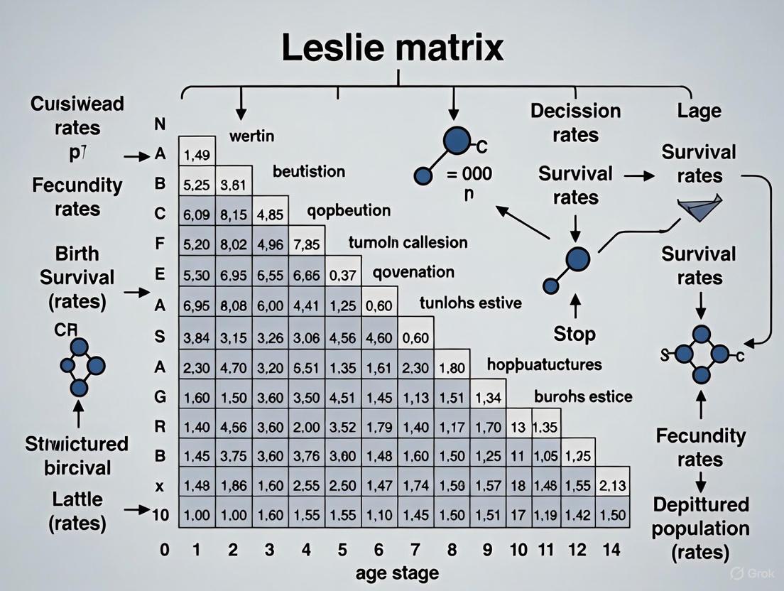
The following diagram illustrates the workflow of constructing and analyzing a Leslie Matrix model.

Application Notes and Protocols

The following sections provide detailed methodologies for applying age-structured models in different research contexts.

Protocol 1: Parameter Estimation for a Wildlife Population Model

Objective: To estimate the parameters of a Leslie matrix for a wild animal population using a combination of field data and literature review.

Materials:

• Field data on survival and fecundity (e.g., from mark-recapture studies, radio telemetry, nest monitoring).
• Demographic data from the literature or species databases (e.g., IUCN, COMPADRE).
• Statistical software (e.g., R, Python with scipy and numpy libraries).

Methodology:

• Define Age Classes: Determine the number of age classes ( k ). This is often based on biological knowledge (e.g., age at first reproduction, maximum lifespan) and data availability. A common approach is to use yearly intervals.
• Estimate Age-Specific Survival Probabilities (( P_x )):
  • Use mark-recapture data analyzed with software such as MARK or the RMark package in R to estimate annual survival probabilities for each age class.
  • Calculate ( Pi ) as the proportion of individuals in age class ( i ) that survive to age class ( i+1 ). For the final age class, ( Pk = 0 ).
• Estimate Age-Specific Fertility Rates (( Fx )):
  • From field studies, determine the average number of female offspring produced per female in each age class.
  • Adjust fertility based on the survival probability of offspring to the first census period. For example, if a female in age class 3 produces 2 offspring on average, and the probability of an offspring surviving to its first birthday is 0.5, then ( F3 = 2 \times 0.5 = 1.0 ).
• Construct the Matrix: Populate the Leslie matrix ( \mathbf{L} ) with the estimated ( Fi ) and ( Pi ) values.
• Validate the Model: If time-series data is available, compare the model's projections against the observed population trends to assess its accuracy and refine parameter estimates.

Protocol 2: Incorporating Age-Structure into an Epidemic Model

Objective: To extend a simple epidemic model to include infection age, demonstrating how the timing of processes like symptom onset and transmission influences outbreak dynamics.

Materials:

• Data on infection rates, incubation periods, and generation intervals from the literature.
• Computational software capable of handling differential equations or matrix algebra (e.g., R, MATLAB, Python).

Methodology:

• Model Selection: Adopt an age-structured Susceptible-Infected-Recovered (SIR) framework, where "age" refers to the time since infection (infection age, ( a )) [2] [3]. A target-cell-limited model with infection age can be described by: [ \frac{dT(t)}{dt} = \lambda - dT(t) - \beta T(t)V(t) ] [ \frac{\partial i(t, a)}{\partial t} + \frac{\partial i(t, a)}{\partial a} = -\delta(a)i(t, a) ] [ \frac{dV(t)}{dt} = \int_0^\infty p(a)i(t, a)da - cV(t) ] where ( i(t, a) ) is the density of infected cells of infection age ( a ) at time ( t ), ( \delta(a) ) is the age-dependent death rate, and ( p(a) ) is the age-dependent viral production rate [2].
• Discretization: Discretize the infection age into classes (e.g., 0-24 hours, 24-48 hours, etc.). The transitions between these classes can be represented in a matrix form analogous to the Leslie matrix, often called a next-generation matrix [3].
• Parameterization: Estimate the distribution of the generation interval (time between infections in a transmission chain) and the incubation period. Use these to inform the values in the discretized model. For example, the probability of transitioning to the next infection-age class can be derived from the rate of progression through the infectious stages.
• Compute the Basic Reproduction Number (( R0 )): Use the spectral radius of the next-generation matrix to calculate ( R0 ), which defines the average number of secondary infections from a single infected individual in a wholly susceptible population [3]. This is a key threshold for predicting epidemic potential.
• Simulation and Analysis: Run simulations to explore how different distributions of infectiousness over the infection age affect the speed and final size of an epidemic. This is critical for evaluating the potential impact of interventions that alter the infection timecourse.

Protocol 3: Model-Informed Drug Development (MIDD)

Objective: To utilize quantitative, often age- or physiology-structured, models to optimize drug development decisions, leading to significant time and cost savings.

Materials:

• Preclinical and clinical pharmacokinetic (PK) and pharmacodynamic (PD) data.
• PBPK (Physiologically-Based Pharmacokinetic) and QSP (Quantitative Systems Pharmacology) modeling software (e.g., GastroPlus, Simbiology, NONMEM, Monolix).

Methodology:

• MIDD Plan Integration: Per standard operating procedures at leading pharmaceutical companies, a MIDD plan is a required component of the Clinical Development Plan (CDP) [4]. This plan outlines the quantitative strategy for informing key development questions.
• Modeling and Simulation: Develop and validate models to inform critical decisions. Common applications include:
  • Population PK Analysis: To understand the sources of variability in drug exposure.
  • Exposure-Response Modeling: To link PK measures to efficacy and safety endpoints.
  • PBPK Modeling: To predict drug-drug interaction potential and support waivers for dedicated clinical trials.
  • Disease Progression Modeling: To characterize the natural history of a disease and the drug's effect on it.
• Impact Assessment and Savings Estimation: Quantify the value of MIDD by estimating cost and time savings. As demonstrated at Pfizer, this can be systematically evaluated by [4]:
  • Cost Savings: Multiply a Per Subject Approximation (PSA) value by the number of subjects saved through trial waivers, "No-Go" decisions, or sample size reductions enabled by modeling.
  • Time Savings: Use benchmark timelines from protocol development to clinical study report availability for waived studies (e.g., ~9 months for a drug-drug interaction study, ~18 months for an organ impairment study).
• Decision Support: Use model outputs to select doses, design efficient clinical trials, predict outcomes, and support regulatory submissions and labeling. Systematic application has yielded annualized average savings of approximately 10 months of cycle time and $5 million per program [4].

Data Presentation: Model Parameters and Outputs

This table defines the core variables and parameters used in the Leslie matrix and related age-structured epidemic models.

Parameter	Definition	Unit	Description & Context
( n_{i,t} )	Number of individuals	Individuals	Count of individuals in age class ( i ) at time ( t ) [1].
( F_i )	Fertility rate	Offspring/individual	Number of female offspring per female in age class ( i ) surviving to next census [1].
( P_i )	Survival probability	Dimensionless	Probability an individual in age class ( i ) survives to age class ( i+1 ) [1].
( \lambda )	Finite rate of increase	Dimensionless	Dominant eigenvalue of Leslie matrix; indicates population growth/decline [1].
( \beta )	Infection rate	mL/(HA·h)	Rate constant for virus infecting target cells in epidemic models [2].
( \delta(a) )	Death rate of infected cells	1/h	Age-dependent mortality rate of infected cells in viral dynamics models [2].
( p(a) )	Virus production rate	HA/cells	Rate of virus production by infected cells of infection age ( a ) [2].
( R_0 )	Basic reproduction number	Dimensionless	Average secondary infections from one infected individual; threshold for epidemic spread [3].

Table 2: Estimated Clinical Trial Savings from Model-Informed Drug Development (MIDD)

Data adapted from a portfolio-level analysis demonstrating the efficiency gains from systematic MIDD application [4].

MIDD Activity Type	Typical Time Saved	Typical Cost Saved	Examples of Trial Types Affected
Phase I Trial Waiver	~9-18 months	$0.4 - $2 million	Bioavailability/Bioequivalence, Drug-Drug Interaction, Hepatic/Renal Impairment
Sample Size Reduction	Varies by study	Varies by PSA and subjects reduced	Phase II/III trials based on exposure-response models
"No-Go" Decision	Full trial timeline	Full trial budget	Program termination based on model predictions of low success probability
Portfolio Average (Per Program)	~10 months	~$5 million	Aggregate annualized savings across a development portfolio

The Scientist's Toolkit: Research Reagent Solutions

Table 3: Essential Reagents and Materials for Age-Structured Model Validation

This table lists key biological and computational tools used in the development and validation of age-structured models in experimental biology.

Item Name	Function/Application	Specifics/Examples
Mark-Recapture Kits	Estimation of age-specific survival probabilities (( P_x )) in wildlife populations.	Includes tags (e.g., PIT tags, bird bands), receivers, and software for data analysis (e.g., Program MARK).
PCR Assays	Pathogen detection and load quantification for parameterizing age-structured epidemic models (e.g., ( p(a) ), ( \delta(a) )).	Specific primers/probes for the target pathogen; used to measure viral production and clearance in infected hosts.
Cell Lines & Virus Stocks	In vitro validation of viral dynamics models; used to estimate infection rate (( \beta )) and viral production parameters.	Well-characterized lines (e.g., MDCK for influenza) and titrated virus stocks for controlled infection experiments [2].
PK/PD Assay Kits	Quantification of drug concentration and biomarkers in biological samples for MIDD.	ELISA, MSD, or LC-MS/MS kits to generate data for population PK and exposure-response modeling.
Computational Software	Construction, parameterization, and analysis of Leslie matrices and other structured models.	R, Python (with numpy, scipy), MATLAB; specialized packages for PBPK (GastroPlus) and population modeling (NONMEM).
Protein Design Software	In silico design of proteins for synthetic biology projects, requiring optimization of binding affinity.	EVOLVE workflow (Python-based), Rosetta; used for in silico mutagenesis and functional prediction [2].

Advanced Visualization: Model Structure and Workflows

The following diagram maps the logical structure and state transitions in an age-structured infection dynamics model, highlighting the key processes and rates.

Patrick H. Leslie's work in the 1940s marked a revolutionary turning point in mathematical demography and population ecology. His 1945 publication, "On the use of matrices in certain population mathematics," together with subsequent papers in 1948, introduced the Leslie Matrix—a discrete, age-structured model of population growth that has become a cornerstone of population biology [5] [6]. This innovation addressed a critical limitation of earlier population models by incorporating population structure, specifically age classes, thereby enabling more realistic projections of population dynamics.

Leslie's model diverged significantly from the earlier geometric and logistic growth models that assumed homogeneous populations without age structure [1]. By considering only one sex (typically females) and assuming a closed population without migration growing in an unlimited environment, the Leslie matrix provided a mathematically tractable yet powerful framework for projecting population changes over time [6]. The model's elegance lies in its ability to use relatively simple matrix algebra to describe complex population dynamics, making it accessible to ecologists and demographers alike.

Seventy-five years after its introduction, the Leslie matrix remains fundamentally important across diverse disciplines including ecology, evolution, and conservation biology [5]. Its applications have expanded to encompass a wide range of taxonomic groups, from humans and whales to plants, bacteria, and even viruses, testifying to the robustness and flexibility of Leslie's original formulation.

The Leslie Matrix: Mathematical Foundation

Core Model Structure

The Leslie matrix model describes population growth through discrete time intervals, with the population structured into discrete age classes. The model requires three fundamental types of data for each age class: the number of individuals, age-specific fertility rates, and age-specific survival rates [6].

Let the population be divided into (ω) age classes. The population at time (t) is represented by a vector:

[ \mathbf{nt} = \begin{bmatrix} n{0} \ n{1} \ n{2} \ \vdots \ n{ω-1} \end{bmatrix}{t} ]

where (n_{i}) represents the number of individuals in age class (i) at time (t).

The Leslie matrix L is a square matrix of dimension (ω×ω):

[ L = \begin{bmatrix} f{0} & f{1} & f{2} & \ldots & f{ω-2} & f{ω-1} \ s{0} & 0 & 0 & \ldots & 0 & 0 \ 0 & s{1} & 0 & \ldots & 0 & 0 \ 0 & 0 & s{2} & \ldots & 0 & 0 \ \vdots & \vdots & \vdots & \ddots & \vdots & \vdots \ 0 & 0 & 0 & \ldots & s_{ω-2} & 0 \end{bmatrix} ]

where (fx) denotes the fertility rate for age class (x) (number of female offspring per female in that age class), and (sx) represents the survival rate from age class (x) to (x+1) [6].

The population projection is calculated as:

[ \mathbf{n{t+1}} = L \cdot \mathbf{nt} ]

This recursive relationship can be extended to project the population multiple time steps into the future:

[ \mathbf{nt} = L^t \cdot \mathbf{n0} ]

where (\mathbf{n_0}) is the initial population vector [6].

Key Parameters and Their Ecological Interpretation

Table 1: Key parameters in the Leslie matrix model

Parameter	Symbol	Ecological Interpretation	Matrix Position
Fertility rate	(f_x)	Number of female offspring per female in age class (x)	First row
Survival rate	(s_x)	Probability of surviving from age class (x) to (x+1)	Subdiagonal
Population vector	(\mathbf{n_t})	Number of individuals in each age class at time (t)	N/A
Finite rate of increase	(\lambda)	Population growth rate per time step	Dominant eigenvalue

The fertility rates (fx) are calculated as (fx = sx \cdot b{x+1}), where (b_{x+1}) represents the per capita birth rate [6]. This formulation accounts for the fact that reproduction typically occurs before mortality within each time step.

Practical Application: Protocols and Workflows

Data Collection and Life Table Construction

The construction of an accurate Leslie matrix begins with the development of a comprehensive life table. The following protocol outlines the standardized methodology for data collection and matrix construction:

Protocol 1: Life Table Construction and Parameter Estimation

• Define Age Classes: Determine the appropriate width and number of age classes based on the species' life history. For most applications, annual intervals are appropriate, though shorter intervals may be used for fast-growing species.

• Census Data Collection:

  • Conduct longitudinal monitoring of marked individuals to track survival and reproduction
  • For each age class, record: number of individuals, number surviving to next age class, number of offspring produced
  • Ensure sufficient sample sizes for robust parameter estimation

• Calculate Vital Rates:

  • Compute age-specific survival rates: (sx = \frac{n{x+1}}{n_x})
  • Compute age-specific fertility rates: (fx = \frac{\text{number of offspring from age class x}}{nx})
  • Apply statistical smoothing if sample sizes are small or data are noisy

• Matrix Validation:

  • Verify that all elements are non-negative
  • Confirm that survival probabilities range between 0 and 1
  • Check for logical consistency in fertility patterns across age classes

Case Study: Sheep Population in New Zealand

Table 2: Vital rates for a sheep population in New Zealand [7]

Age (years)	Birth Rate	Survival Rate	Calculated fx
0-1	0.000	0.845	0.000
1-2	0.045	0.975	0.045
2-3	0.391	0.965	0.391
3-4	0.472	0.950	0.472
4-5	0.484	0.926	0.484
5-6	0.546	0.895	0.546
6-7	0.543	0.850	0.543
7-8	0.502	0.786	0.502
8-9	0.468	0.691	0.468
9-10	0.459	0.561	0.459
10-11	0.433	0.370	0.433
11-12	0.421	0.000	0.421

For this sheep population, the resulting Leslie matrix has the following structure:

[ L = \begin{bmatrix} 0.000 & 0.045 & 0.391 & 0.472 & 0.484 & 0.546 & 0.543 & 0.502 & 0.468 & 0.459 & 0.433 & 0.421 \ 0.845 & 0 & 0 & 0 & 0 & 0 & 0 & 0 & 0 & 0 & 0 & 0 \ 0 & 0.975 & 0 & 0 & 0 & 0 & 0 & 0 & 0 & 0 & 0 & 0 \ 0 & 0 & 0.965 & 0 & 0 & 0 & 0 & 0 & 0 & 0 & 0 & 0 \ 0 & 0 & 0 & 0.950 & 0 & 0 & 0 & 0 & 0 & 0 & 0 & 0 \ 0 & 0 & 0 & 0 & 0.926 & 0 & 0 & 0 & 0 & 0 & 0 & 0 \ 0 & 0 & 0 & 0 & 0 & 0.895 & 0 & 0 & 0 & 0 & 0 & 0 \ 0 & 0 & 0 & 0 & 0 & 0 & 0.850 & 0 & 0 & 0 & 0 & 0 \ 0 & 0 & 0 & 0 & 0 & 0 & 0 & 0.786 & 0 & 0 & 0 & 0 \ 0 & 0 & 0 & 0 & 0 & 0 & 0 & 0 & 0.691 & 0 & 0 & 0 \ 0 & 0 & 0 & 0 & 0 & 0 & 0 & 0 & 0 & 0.561 & 0 & 0 \ 0 & 0 & 0 & 0 & 0 & 0 & 0 & 0 & 0 & 0 & 0.370 & 0 \ \end{bmatrix} ]

Population Projection and Analysis Protocol

Protocol 2: Population Projection and Stable Structure Analysis

• Initial Population Setup:

  • Define initial population vector (\mathbf{n_0}) with known or estimated age distribution
  • Normalize if working with proportional age distributions

• Matrix Multiplication:

  • For each time step, compute (\mathbf{n{t+1}} = L \cdot \mathbf{nt})
  • Implement in computational environment (R, Python, MATLAB) for multiple iterations

• Long-term Behavior Analysis:

  • Compute dominant eigenvalue (\lambda_1) of Leslie matrix
  • Compute corresponding right eigenvector (\mathbf{w}) (stable age distribution)
  • Compute corresponding left eigenvector (\mathbf{v}) (reproductive value)

• Interpretation:

  • If (\lambda_1 > 1): population increasing
  • If (\lambda_1 = 1): population stable
  • If (\lambda_1 < 1): population decreasing
  • Stable age distribution: (\mathbf{w}) normalized to sum to 1

The computational workflow for implementing and analyzing a Leslie matrix model can be visualized as follows:

Extensions and Contemporary Applications

Evolution of Structured Population Models

While Leslie's original model considered age as the only structuring variable, subsequent developments have expanded this framework significantly. The most notable extension is the Lefkovitch matrix, which replaces age classes with ontogenetic stages, allowing individuals to remain in the same stage class or move to the next one [6]. This approach is particularly valuable for species where development depends more on size or life stage than chronological age.

Continuous-time formulations of structured population models were first introduced in the pioneering works of Sharpe and Lotka (1911) and McKendrick (1926), who considered age as the only structuring variable [8]. Later, Gurtin and MacCamy (1974) developed a non-linear age-structured model that allowed mortality and fertility rates to be affected by total population size, introducing density-dependence to the framework [8].

Modern structured population models typically involve systems of first-order hyperbolic partial integro-differential equations for the time-dependent density function with respect to the chosen structuring variables [8]. These models have become essential tools in diverse fields including demography, epidemiology, ecology, cell kinetics, and tumor growth.

Contemporary Research Applications

Table 3: Contemporary applications of matrix population models

Application Area	Specific Use	Key Advancements
Conservation Biology	Population viability analysis for endangered species	Incorporation of stochasticity, sensitivity analysis
Climate Change Research	Predicting species responses to changing environments	Integration of environmental drivers, transient dynamics
Eco-evolutionary Dynamics	Studying hybridization and genome extinction	Multi-species matrix models, eco-evolutionary feedbacks
Insect Demography	Understanding host-parasite interactions	Stage-structured models, experimental validation
Epidemiology	Disease spread in structured populations	Age-structured SIR models, contact matrices

Recent research has demonstrated the expanding utility of Leslie's foundational framework. For example, Santostasi et al. (2020) applied matrix models to study hybridization and genome extinction in wolf and dolphin populations, providing insights into conservation strategies for hybridizing species [5]. Similarly, Davison et al. (2019) applied stochastic Life Table Response Experiments (sLTRE) to 220 populations from 62 species, finding that stochasticity drives 28% of fitness effects—exceeding mean effects by 7.78%—highlighting the importance of incorporating environmental variability in population projections [5].

The Scientist's Toolkit: Research Reagent Solutions

Table 4: Essential research reagents and computational tools for matrix population modeling

Tool Category	Specific Tool/Software	Function/Purpose
Data Collection Tools	Mark-recapture kits, Field monitoring equipment, Genetic sampling kits	Collect survival and reproduction data in field conditions
Statistical Software	R (popbio, popdemo packages), MATLAB, Python (NumPy, SciPy)	Matrix construction, population projection, eigenanalysis
Specialized Packages	R: popbio for matrix analysis, popdemo for demographic analysis, IPMpack for integral projection models	Implementation of specialized demographic analyses
Visualization Tools	ggplot2 (R), matplotlib (Python), Graphviz for workflow diagrams	Data visualization, model output presentation
Database Resources	COMADRE (animal populations), COMPADRE (plant populations)	Access to published matrix population models for comparative studies

The computational tools listed in Table 4 represent the modern evolution of Leslie's original computational approach. While Leslie worked with matrix algebra on paper or early calculators, contemporary researchers leverage sophisticated statistical software and specialized packages that implement the same fundamental mathematics with greater efficiency and expanded analytical capabilities.

Patrick Leslie's contribution to population ecology represents a paradigm shift in how biologists approach population modeling. By introducing age structure through matrix algebra, he provided a mathematically rigorous yet practical framework that has stood the test of time. The Leslie matrix remains fundamentally important 75 years after its introduction, continuing to inspire new developments in mathematical ecology and conservation biology.

The enduring legacy of Leslie's work is evident in its expansion to diverse taxonomic groups, its adaptation to various structuring variables beyond age, and its integration with eco-evolutionary dynamics. As population ecologists face new challenges related to global change, biodiversity loss, and emerging diseases, the Leslie matrix continues to provide a robust foundational framework for understanding and predicting population dynamics in an increasingly variable world.

The Leslie matrix is a foundational tool in population ecology, providing a discrete, age-structured model of population growth. First introduced by P.H. Leslie in 1945, this mathematical construct projects population dynamics over time by leveraging two fundamental biological parameters: age-specific fecundity and survival rates [6]. The model's enduring relevance lies in its ability to translate individual-level vital rates into population-level projections, making it invaluable for predicting population growth, stability, and age-structure evolution. Within broader thesis research on age-structured populations, understanding the precise role and quantification of these core components is paramount for ecological risk assessments, conservation planning, and evolutionary studies, including investigations into life history strategies such as semelparity versus iteroparity [9] [10].

This article details the core components of Leslie matrices, providing application notes and experimental protocols for researchers aiming to construct and utilize these models in population biology, ecological risk assessment, and evolutionary studies.

Core Principles and Mathematical Formulation

The Leslie model represents a population closed to migration, growing in an unlimited environment, and typically considers only the female segment of a population [6]. The population is divided into discrete age classes, and its state at any time ( t ) is represented by a vector ( \mathbf{n_t} ).

The Population Projection Equation

The fundamental equation projecting the population from one time step to the next is:

[ \mathbf{n{t+1}} = \mathbf{L} \mathbf{nt} ]

where ( \mathbf{n_t} ) is the population vector at time ( t ), and ( \mathbf{L} ) is the Leslie projection matrix [6]. After ( t ) time steps, the population state derives from:

[ \mathbf{nt} = \mathbf{L^t} \mathbf{n0} ]

where ( \mathbf{n_0} ) is the initial population vector [6].

Structure of the Leslie Matrix

The Leslie matrix ( \mathbf{L} ) is a square matrix with a specific structure. For a population with ( \omega ) age classes, the matrix is defined as follows [6]:

[ L = \begin{bmatrix} f0 & f1 & f2 & \ldots & f{\omega-2} & f{\omega-1} \ s0 & 0 & 0 & \ldots & 0 & 0 \ 0 & s1 & 0 & \ldots & 0 & 0 \ 0 & 0 & s2 & \ldots & 0 & 0 \ \vdots & \vdots & \vdots & \ddots & \vdots & \vdots \ 0 & 0 & 0 & \ldots & s_{\omega-2} & 0 \end{bmatrix} ]

• Top Row ((f_x)): Contains the age-specific fecundity coefficients, representing the average number of female offspring produced per female in age class ( x ), surviving to the next census period.
• Sub-diagonal ((s_x)): Contains the age-specific survival probabilities, representing the fraction of individuals in age class ( x ) that survive to age class ( x+1 ) at the next time step.
• All other elements: Are zero, reflecting the deterministic progression of individuals from one age class to the next [6].

Quantitative Parameters: Fecundity and Survival

The accuracy of any Leslie model hinges on the correct estimation of its fecundity and survival parameters. The table below summarizes the core data required to construct the matrix.

Table 1: Core Data Components for Constructing a Leslie Matrix

Parameter	Symbol	Description	Measurement Unit	How Obtained
Number of Individuals	( n_x )	Count of females in each age class ( x ) at time ( t ) [6].	Individuals	Field census, laboratory count [11].
Survival Probability	( s_x )	Fraction of individuals of age ( x ) that survive to age ( x+1 ) [6].	Unitless (0 to 1)	Longitudinal tracking, mark-recapture studies, life table analysis [11].
Average Female Offspring	( m_x )	Average number of female offspring produced per female of age ( x ) (also called fertility rate) [11].	Offspring per female	Field observation, controlled breeding experiments [11].
Fecundity Coefficient	( f_x )	Number of female offspring per female of age ( x ) that survive to the next census point. It integrates fertility and infant survival [6].	Offspring per female	Calculated as ( fx = sx \cdot b{x+1} ), where ( b{x+1} ) is the birth rate, or directly from ( n_0 ) data [6].

The relationship between fertility (( mx )) and the fecundity coefficient (( fx )) used in the matrix is critical. The fecundity coefficient is calculated as ( fx = sx \cdot b{x+1} ), where ( b{x+1} ) is the birth rate, or is derived directly from data on the number of newborns (( n0 )) [6]. In a pre-breeding census model, ( fx ) effectively represents the number of female offspring, born to mothers of age ( x ), that survive to be counted in the first age class at the next time step [10] [6].

Experimental Protocol for Model Construction and Application

This protocol provides a step-by-step methodology for building a Leslie matrix from raw demographic data and using it for population projection, adaptable for both field and laboratory settings.

The diagram below outlines the logical workflow for constructing and applying a Leslie Matrix model.

Step-by-Step Procedure

Step 1: Define Age Classes and Conduct Initial Census

• Determine the number of age classes (( \omega )) and the duration of each time step (e.g., one year) based on the organism's life history [11].
• Conduct a census of the population. Record the number of female individuals (( nx )) in each age class ( x ), where ( x = 0, 1, 2, ..., \omega-1 ). This forms your initial population vector, ( \mathbf{n0} ) [11].

Step 2: Estimate Age-Specific Survival Probabilities (( s_x ))

• Longitudinal Tracking: Track a cohort of individuals over time. The survival probability from age ( x ) to ( x+1 ) is calculated as: [ s_x = \frac{\text{Number of individuals alive at age } x+1}{\text{Number of individuals alive at age } x} ]
• Life Table Analysis: Use a life table to calculate ( lx ), the proportion of newborns surviving to age ( x ). Then, ( sx = l{x+1} / lx ) [11].

Step 3: Estimate Age-Specific Fertility (( m_x ))

• For each age class ( x ), record the average number of female offspring produced per female over one time step. This is the fertility rate, ( m_x ) [11].
• These data are typically collected through controlled breeding experiments or intensive field observation.

Step 4: Calculate Fecundity Coefficients (( f_x )) for the Matrix

• The fecundity coefficient (( f_x )) used in the top row of the Leslie matrix must account for offspring survival to the first census point.
• A common calculation is ( fx = sx \cdot b{x+1} ), where ( b{x+1} ) is the birth rate, or it can be derived directly from data on the number of newborns (( n0 )) [6]. In many practical models, the fertility rate ( mx ) is used directly as a proxy for ( f_x ) if offspring are censused immediately after birth [11].

Step 5: Construct the Leslie Matrix

• Create a square matrix of dimension ( \omega \times \omega ).
• Populate the first row with the fecundity coefficients ( f0, f1, ..., f_{\omega-1} ).
• Populate the sub-diagonal with the survival probabilities ( s0, s1, ..., s_{\omega-2} ).
• Set all other matrix elements to zero [6] [11].

Step 6: Project Population Dynamics

• Initialize the model with the population vector ( \mathbf{n_0} ).
• Project the population by iteratively multiplying the current population vector by the Leslie matrix: [ \mathbf{n1} = L \mathbf{n0}, \quad \mathbf{n2} = L \mathbf{n1} = L^2 \mathbf{n_0}, \quad \text{etc.} ]
• Analyze the results for total population size, age structure, and growth rate over time [11].

Advanced Applications and Modifications

The basic Leslie model can be extended to address more complex ecological and evolutionary questions.

Incorporating Density Dependence and Competition

The classic Leslie model generates exponential growth or decay. For realism, density dependence must be added, where survival and/or fecundity decrease as the population grows. The Leslie Logistic Model incorporates this by making vital rates functions of population density [9]. Furthermore, Projection of Interspecific Competition (PIC) Matrices have been developed to model population dynamics of two or more species competing for shared resources, addressing a major limitation of the single-species Leslie model [10].

Evolutionary Dynamics: The Darwinian Extension

The Leslie framework can be merged with evolutionary game theory to create Darwinian matrix models. These models allow a heritable phenotypic trait to evolve subject to natural selection, with fitness consequences determined through the Leslie matrix's vital rates. This approach can be used to investigate the evolution of life-history strategies, such as the conditions favoring semelparity (a single reproductive event) versus iteroparity (multiple reproductive events) [9].

The Scientist's Toolkit: Essential Reagents and Materials

Table 2: Key Research Reagent Solutions for Demographic Studies

Item	Function/Application in Leslie Matrix Research
Field Mark-Recapture Kits	Essential for estimating age-specific survival probabilities (( s_x )) in wild populations. Includes tags, bands, transmitters, and detection equipment.
Genetic Sexing Assays	Critical for accurately determining the sex ratio of offspring and the adult population, ensuring accurate calculation of female-specific fecundity (( mx ), ( fx )).
Laboratory Animal Colonies	Provide controlled environments for precise measurement of survival and fecundity parameters under constant or experimental conditions (e.g., toxicant exposure [10]).
Statistical & Modeling Software	Used for matrix construction, matrix algebra operations (eigenanalysis), population projection, and visualization of results (e.g., age-structure pyramids, growth curves).
Life Table Analysis Tools	Software or computational scripts to convert raw census data into life tables, from which ( lx ), ( sx ), and other key metrics are derived [11].

Key Assumptions and Limitations of the Basic Leslie Model

The Leslie Matrix Model is a foundational tool in population ecology, providing a discrete, age-structured framework for projecting population dynamics over time. First introduced by P. H. Leslie in 1945, this approach represents a significant advancement over simpler, unstructured population models by accounting for how birth and death rates vary with age [1] [12]. The model projects population changes using a recurrence relation where the population state vector at time t+1 is determined by multiplying a square matrix (the Leslie matrix) by the population state vector at time t: N(t+1) = A × N(t) [1] [13]. As time progresses, the population typically converges to a stable age distribution and grows at a constant exponential rate, λ, which is the dominant eigenvalue of the Leslie matrix [1] [13]. This model serves as a critical component in conservation biology, resource management, and evolutionary studies, particularly for evaluating species' responses to environmental pressures and informing management strategies [14] [12]. This document outlines the core assumptions, limitations, and validation protocols essential for the proper application of the basic Leslie model in research contexts.

Core Assumptions of the Basic Leslie Model

The mathematical structure of the Leslie model relies on several fundamental assumptions, which, if violated, can compromise the accuracy and reliability of its projections.

• Assumption 1: Constant Vital Rates. The model assumes that age-specific survival and fertility rates remain constant over time, leading to deterministic, exponential growth [1]. In reality, vital rates are subject to temporal variability due to environmental fluctuations, rendering this assumption tenable only for short-term projections in stable environments.
• Assumption 2: Unlimited Resources. The model projects unconstrained geometric growth, implicitly assuming that resources such as space and food are virtually unlimited [1]. It does not account for density-dependent feedback mechanisms that regulate population size, a significant limitation for populations near their environmental carrying capacity [12].
• Assumption 3: Discrete Age Classes and Time Intervals. Individuals are grouped into discrete age classes (e.g., 0-1 years, 1-2 years), and population transitions are calculated at discrete time intervals [1]. This requires that the age classes and time steps be synchronized, which can be problematic for species with continuous reproduction or non-annual life cycles.
• Assumption 4: Single-Sex Population. The classic model typically tracks only one sex, usually the female, and assumes that male availability does not limit reproduction [1]. This ignores potential Allee effects and mate limitations, which can be critical in small or declining populations.
• Assumption 5: Population Closure. The model assumes a closed population, meaning it completely ignores the effects of immigration and emigration on population dynamics [1]. This restricts its applicability to populations that are geographically or reproductively isolated.

The following diagram illustrates the logical workflow and the critical decision points based on these core assumptions when constructing a Leslie model.

Key Limitations and Common Errors

Despite its utility, the Leslie model has inherent limitations, and its application in scientific literature is frequently marred by specific, recurring construction errors.

Inherent Model Limitations

• Deterministic and Density-Independent Projections: The basic model cannot simulate population fluctuations driven by environmental stochasticity or density-dependent regulation, which are fundamental aspects of real-world population dynamics [1] [12].
• Transient Dynamics Overshadowed: The model's asymptotic behavior (λ and stable age distribution) often receives the most attention, while transient dynamics—the population's short-term response to perturbation—are overlooked, despite being critical for conservation planning [14].
• Sensitivity to Parameter Uncertainty: Model predictions are highly sensitive to the accuracy of its vital rates. These rates are often estimated with sampling uncertainty, which propagates through the model and can lead to imprecise or biased estimates of the population growth rate (λ) [13].

Prevalent Construction Errors

Empirical analysis of studies within the COMADRE Animal Matrix Database reveals that errors in model construction are widespread [15].

• Fertility Coefficient Error: A common error is the failure to include survival in the fertility coefficient. The number of newborns produced by an age class must account for the mother's survival to that age class. This error was found in 34% of examined studies using a post-breeding census [15].
• Reproduction Timing Error: Many models incorrectly introduce a one-year delay in the age of first reproduction, misaligning the life cycle with the population census timing. This was the most frequent error, appearing in 62% of relevant studies [15].
• Growth Rate Calculation Error: In models where stages (or age classes with prolonged duration) are used, inappropriate formulas are often applied to calculate the asymptotic population growth rate or its sensitivity. This error was identified in 53% of studies where stages could last more than one time step [15].

Table 1: Prevalence of Common Construction Errors in Published Leslie Matrix Models (based on [15])

Error Type	Description	Prevalence in Published Studies
Fertility Coefficient Error	Failing to incorporate maternal survival into the fecundity term.	34%
Reproduction Timing Error	Incorrectly delaying the age at first reproduction by one time step.	62%
Growth Rate Calculation Error	Using wrong formulas for asymptotic growth or sensitivity analysis.	53%

Experimental Protocol for Model Construction and Validation

This protocol provides a step-by-step guide for building and validating a basic, age-structured Leslie Matrix model, incorporating checks to avoid common errors.

The experimental workflow for constructing and validating a Leslie model involves sequential stages of data collection, matrix construction, analysis, and validation, as visualized below.

Step-by-Step Procedure

Phase 1: Data Collection and Life Table Creation

• Define Age Classes: Establish discrete, consecutive age classes (x) that align with the species' life history and the chosen projection time step (e.g., years) [1] [11].
• Census Initial Population: Count the number of individuals (nₓ) in each age class at the starting time (t=0) [11].
• Estimate Vital Rates:
  • Survival Probability (sₓ): For each age class x, calculate the fraction of individuals that survive from the start of age class x to the start of age class x+1. This often requires mark-recapture or longitudinal cohort data [11].
  • Fecundity (mₓ): Determine the average number of female offspring produced per female in age class x that survive to the next census point. This is a critical step where Error 1 (Fertility Coefficient) commonly occurs; ensure mₓ accounts for offspring survival to the census point if necessary [15] [11].

Phase 2: Leslie Matrix Construction

• Matrix Structure: Construct a square matrix with dimensions equal to the number of age classes, k.
• Populate Subdiagonal (Survival Elements): Place the age-specific survival probability sₓ in the cell below the main diagonal for each row i (i.e., position A[i+1, i]). This transitions individuals from age class i to i+1 [1] [11].
• Populate First Row (Fertility Elements): Calculate the fertility coefficient fₓ for the first row. This is where Error 2 (Reproduction Timing) must be avoided. For a pre-breeding census, fₓ = s₀ × mₓ, where s₀ is newborn survival. For a post-breeding census, fₓ = mₓ₊₁, as births occur after the census and are attributed to the age of the mother at the next time step [15] [11].
• Set All Other Elements to Zero: All remaining cells in the matrix should be zero.

Phase 3: Model Analysis and Projection

• Population Projection: Multiply the Leslie matrix by the initial population vector to project the population forward in time: N(t+1) = L × N(t). Iterate for multiple time steps [1] [11].
• Calculate Asymptotic Properties:
  • Finite Rate of Increase (λ): Calculate the dominant eigenvalue of the Leslie matrix. This represents the asymptotic population growth rate (λ > 1 indicates growth, λ < 1 indicates decline) [1] [13].
  • Stable Age Distribution: Calculate the corresponding right eigenvector, which represents the proportion of individuals in each age class toward which the population converges over time [14] [1].
  • Reproductive Value: Calculate the left eigenvector, which quantifies the expected contribution of an individual in a given age class to future population growth [14].

Phase 4: Sensitivity, Uncertainty, and Validation

• Sensitivity and Elasticity Analysis: Perform these analyses to determine how changes in specific vital rates (survival and fecundity) affect λ. This identifies which life history stages have the greatest impact on population growth. Be cautious to avoid Error 3 (Growth Rate Calculation) by using established formulas for sensitivity of λ to matrix elements [14] [15].
• Uncertainty Analysis: Use bootstrapping or analytic methods to estimate confidence intervals for λ, acknowledging the sampling error in the underlying vital rate estimates [13].
• Model Validation: Where possible, compare model projections with subsequent, independently observed population trends to assess predictive accuracy.

This section details essential data sources, software, and analytical concepts required for constructing and analyzing Leslie matrix models.

Table 2: Essential Resources for Leslie Matrix Modeling

Resource / Concept	Type	Function and Application
FishBase / FishLife	Database / R Package	Provides life history data (growth, mortality, fecundity) for parameterizing models of data-deficient fish species [14].
COMADRE Database	Database	A repository of published matrix population models for animals; useful for comparative studies and verifying model structure [15].
Bootstrap Resampling	Statistical Method	A computational technique for estimating confidence intervals and sampling uncertainty for model outputs like λ [13].
Sensitivity & Elasticity	Analytical Metric	Quantifies the relative importance of vital rates to population growth, guiding targeted management interventions [14].
Damping Ratio	Population Metric	Measures how quickly a population returns to its stable age distribution after a disturbance; informs on transient dynamics [14].
R / Python	Programming Language	Provides flexible environments (with packages like 'popbio' in R) for matrix construction, projection, and eigenvalue analysis [14] [16].
Pre-breeding vs. Post-breeding Census	Conceptual Framework	Defines the timing of the population census relative to the birth pulse, which dictates the correct formulation of fertility coefficients [15].

The Leslie matrix model remains an indispensable tool for understanding the dynamics of age-structured populations. Its effective application, however, is contingent upon a rigorous adherence to its underlying assumptions and a meticulous approach to model construction. Researchers must be vigilant of the common pitfalls detailed herein, particularly those related to fertility calculation, reproductive timing, and growth rate analysis. By employing the standardized protocols, validation checks, and resources outlined in this document, scientists can enhance the reliability of their models, thereby producing more accurate and impactful insights for conservation, management, and evolutionary ecology. Future work should focus on integrating density-dependence, environmental stochasticity, and evolutionary dynamics to extend the utility of this classic framework [12].

In biomedical research, accurately modeling biological processes and intervention outcomes is fundamental to advancing therapeutic development. Population models, which mathematically describe changes in populations over time, serve as critical tools in this endeavor. Unstructured population models treat the population as a homogeneous unit, tracking only total numbers and ignoring internal individual variation. In contrast, age-structured population models, principally implemented through Leslie matrices, explicitly partition a population into discrete age classes and track the number of individuals in each class over time [17]. This fundamental difference confers significant and measurable advantages for biomedical applications, particularly in aging research, drug development, and personalized medicine. The ability to incorporate age-specific vital rates—such as survival, fecundity, and mortality—allows researchers to move beyond population-level averages and capture the profound heterogeneity inherent in biological systems [18] [17].

The Leslie matrix model projects an age-structured population forward in time via a matrix multiplication operation. The population at time t is represented by a vector nt, and the model is described by the equation: n{t+1} = L * n_t, where L is the Leslie matrix containing age-specific survival and fecundity values [17]. This structured approach is uniquely powerful for simulating the long-term demographic consequences of age-dependent phenomena, a common scenario in disease progression and therapeutic intervention.

Figure 1: Leslie Matrix Model Workflow. The model projects the population forward by multiplying the current population vector by the Leslie matrix, which is built from age-specific fecundity and survival parameters.

Comparative Analysis: Structured vs. Unstructured Models

The choice between structured and unstructured modeling approaches has profound implications for the predictive power and applicability of a model in a biomedical context. The core distinction lies in their treatment of population heterogeneity.

Unstructured models, such as the exponential or logistic growth models, utilize a single, often simplistic, equation to describe the growth of the entire population. They operate on the average properties of the population, implicitly assuming all individuals are identical and equally likely to reproduce or die. This can lead to significant inaccuracies when these assumptions are violated, which is the norm in biological systems.

Structured models, specifically the age-structured Leslie matrix, fundamentally reject this homogeneity. They classify individuals into state classes (e.g., age, life stage, health status) and define state-specific transition probabilities. This allows for a nuanced representation where outcomes—such as the probability of reproducing, succumbing to a disease, or responding to a treatment—are dependent on an individual's state.

Table 1: Quantitative Comparison of Model Attributes

Model Attribute	Unstructured Model	Leslie Matrix (Age-Structured)
Population Representation	Single, homogeneous unit	Disaggregated into multiple age classes
Key Parameters	Global growth rate (r), carrying capacity (K)	Age-specific survival (sx), fecundity (fx)
Data Requirements	Lower (total population counts)	Higher (age-class-specific vital rates) [17]
Projection Output	Total population size only	Total population size and age distribution [17]
Stable Age Distribution	Not applicable; assumed instantaneous	Can be derived from the matrix (dominant eigenvector) [17]
Sensitivity Analysis	Limited to global parameters	Can pinpoint critical, sensitive age classes [17]

The advantages of the Leslie matrix extend beyond simply tracking age structure. A key analytical derivative is the stable age distribution, which is the population's eventual age composition, and the finite rate of population change (λ), representing the intrinsic growth rate. These are derived from the matrix's dominant eigenvector and eigenvalue, respectively [17]. Furthermore, sensitivity and elasticity analyses can be performed on the Leslie matrix to determine which age-specific vital rates (e.g., survival of juveniles vs. fecundity of adults) have the strongest influence on population growth. This is invaluable for identifying optimal intervention points in disease management or conservation efforts [17].

Advantages of Leslie Matrices in Key Biomedical Applications

Aging Research and Intervention Testing

The Leslie matrix is exceptionally suited for aging research because it directly incorporates the core variable of interest: age. It can model the demographic consequences of interventions that differentially affect various life stages.

For example, a therapy that delays aging by reducing mortality rates across all ages, versus one that specifically enhances survival in old age, will have distinct impacts on the population's age structure and growth rate. The Leslie matrix can quantitatively project these differences, something unstructured models are incapable of doing. This is critical in an era where research into "healthspan"—the period of life spent in good health—is prioritized alongside lifespan [19]. Models can be used to project not just the number of individuals alive, but the shifting demographic burden and the prevalence of age-related diseases, informing public health and drug development strategies.

Preclinical Modeling of Therapeutic Efficacy and Toxicity

In drug development, Leslie matrices provide a framework for integrating preclinical data on age-dependent drug effects. A therapeutic candidate might show high efficacy in mature adults but cause toxicity in developing juveniles, or its mechanism of action might be inherently linked to a specific biological process active only in certain life stages.

• Integrating Complex Exposure Scenarios: As demonstrated in ecological risk assessment, Leslie matrices can analyze scenarios where different life stages are concurrently exposed to a stressor [18]. Translated to biomedicine, this allows for modeling a drug's effect when administered to a population containing both adults and developing individuals, projecting outcomes on total population size and the recruitment of the next (F1) generation in preclinical animal studies.
• Linking Mechanism to Population Outcome: The model's structure allows for the integration of effects acting via different molecular pathways at different life stages [18]. For instance, a drug might inhibit a specific enzyme in adults (an "activational" effect) but alter developmental programming when exposure occurs in utero (an "organizational" effect). The Leslie matrix can synthesize these disparate data to predict the net population-level consequence.

Analysis of Demographic Shifts and Disease Burden

Globally, populations are undergoing a massive demographic shift towards an older age structure [19]. This has profound implications for the prevalence of chronic, age-related diseases. Leslie matrices, unlike unstructured models, are powerful tools for forecasting this changing age distribution and its associated disease burden. By projecting the proportion of the population in older age classes, researchers and policymakers can better anticipate future healthcare needs and resource allocation for conditions like sarcopenia, neurodegenerative diseases, and metabolic disorders.

Experimental Protocol: Implementing a Leslie Matrix for a Preclinical Study

This protocol details the steps to construct and use a Leslie matrix to model a drug's effect on an aging laboratory animal population.

4.1 Objective: To project the long-term population-level impact of a novel gerotherapeutic drug on a cohort of mice, accounting for its age-specific effects on survival and fecundity.

4.2 Materials and Reagents: Table 2: Research Reagent Solutions and Essential Materials

Item	Function/Description	Application in Protocol
Laboratory Animal Cohort	Inbred strain (e.g., C57BL/6J) or premature aging model (e.g., SAMP8) with known age-specific survival.	Serves as the baseline population; data used to parameterize the control Leslie matrix. [19]
Candidate Therapeutic	Small molecule (e.g., thymol, carvacrol [20]), biologic, or other intervention.	The independent variable; its age-specific effects on vital rates are to be modeled.
Vital Rates Data	Age-specific survival probability (sx) and fecundity (mx, number of female offspring per female).	The core empirical data required to build the Leslie matrix. Can be obtained from historical colony data or a dedicated longitudinal study.
Computational Software	R, Python (with NumPy/Pandas), or MATLAB.	Used to perform matrix algebra, project the population, and calculate λ and stable age distribution.

4.3 Procedure:

• Define Age Classes: Establish discrete age classes for the model (e.g., 0-3 months, 3-6 months, ..., until maximum lifespan). The time step should match the class width.

• Parameterize the Control Matrix (L_control):

  • Estimate Survival Probabilities (s_x): From control group data, calculate the proportion of individuals in age class x that survive to age class x+1.
  • Estimate Fecundities (f_x): Calculate the average number of female offspring (reaching the first age class) produced per female in age class x. Note: f_x = s_x * m_x+1, where m is the average offspring per female [17].
  • Construct the Matrix: Place f_x values in the first row and s_x values on the sub-diagonal of L_control.

• Parameterize the Treatment Matrix (Ltreatment): Incorporate the drug's effects. For example, if the drug increases survival in older age classes by 20%, multiply the corresponding s_x values in Lcontrol by 1.2 to create L_treatment.

• Initialize the Population Vector (n_0): Create a vector representing the starting number of individuals in each age class.

• Run the Projection: Iteratively multiply the population vector by the Leslie matrix for the desired number of time steps (e.g., until the population reaches a stable growth rate or becomes extinct). n_{t+1} = L * n_t

• Analyze Output:

  • Plot total population size over time for both control and treatment groups.
  • Calculate the finite rate of increase (λ) as the dominant eigenvalue of each Leslie matrix. A λ > 1 indicates a growing population.
  • Compare the stable age distributions (dominant eigenvector) between groups.
  • Perform elasticity analysis to identify which vital rates most influence λ in the control population, indicating potential leverage points for the intervention.

Figure 2: Leslie Matrix Experimental Protocol. A sequential workflow for implementing a Leslie matrix model in a preclinical research context.

The transition from unstructured population models to age-structured Leslie matrices represents a critical evolution in biomedical modeling capability. By explicitly accounting for age-dependent variation in survival, fecundity, and susceptibility, the Leslie matrix framework provides a more biologically realistic and powerful tool for researchers. Its ability to integrate complex, age-specific data, project long-term demographic outcomes, and identify sensitive intervention points makes it indispensable for tackling modern challenges in aging research, therapeutic development, and understanding demographic health trends. As biomedical research continues to emphasize personalized and age-specific medicine, the adoption of structured population models like the Leslie matrix will be fundamental to translating mechanistic discoveries into meaningful health outcomes.

Implementing Leslie Matrices: Step-by-Step Methodology and Research Applications

The Leslie matrix is a foundational tool in population ecology, providing a discrete, age-structured model for projecting population growth. Named after Patrick H. Leslie, this matrix model projects the future state of a population segmented into discrete age classes, based on its current age-specific fertility and survival rates [6]. It is particularly valuable for modeling the dynamics of wildlife populations, evaluating conservation strategies, and assessing the impact of anthropogenic pressures like fisheries bycatch [21]. This protocol details the essential data requirements and methodologies for constructing and implementing a Leslie matrix, providing a standardized guide for researchers.

Data Requirements for Matrix Construction

Constructing an accurate Leslie matrix requires two primary types of age-specific vital rates. The model typically considers only the female segment of a population, assuming it is closed to migration and growing in an unlimited environment [6]. The required parameters are summarized in Table 1.

Table 1: Essential Data Parameters for a Leslie Matrix

Parameter	Symbol	Description	Measurement Units
Age-Specific Fertility Rate	( f_x )	The average number of female offspring born per individual in age class ( x ), surviving to the next census.	Offspring per female per time step
Age-Specific Survival Rate	( s_x )	The probability that an individual in age class ( x ) will survive to age class ( x+1 ).	Unitless (0 to 1)
Number of Age Classes	( \omega )	The maximum age attainable, defining the dimensions of the matrix and population vector.	Number of classes

Parameter Definitions and Calculations

• Age-Specific Fertility (( fx )): This parameter is a composite measure. It is the product of the birth rate (( bx ), the average number of offspring, both male and female, per mother) and the survival probability of the mother over the interval, often adjusted for the sex ratio [6]. Formally, it can be expressed as ( fx = sx b{x+1} ), where ( b{x+1} ) is the average number of female offspring per capita [6].
• Age-Specific Survival (( s_x )): This is the probability of surviving from age class ( x ) to ( x+1 ). It is calculated from empirical life table data or marked individual studies [1] [7].

Experimental Protocols for Parameter Estimation

Accurate parameter estimation is critical for generating reliable population projections. The following protocols outline standard methodologies.

Field Data Collection and Longitudinal Studies

Objective: To empirically estimate age-specific survival and fertility rates through direct observation.

• Study Design: Establish a long-term monitoring program for a marked population. Individuals are captured, marked (e.g., with tags, bands, or transmitters), and their age is recorded at first capture.
• Data Collection:
  • For Survival Rates: Conduct regular recapture or resighting surveys. Record the presence/absence of marked individuals of known age over multiple time steps (e.g., annually).
  • For Fertility Rates: Perform reproductive status surveys. For females in each age class, count the number of offspring produced that survive to the next census period.
• Data Analysis:
  • Survival Analysis: Use statistical models (e.g., Cormack-Jolly-Seber models) on capture-recapture history data to estimate age-specific annual survival probabilities (( sx )).
  • Fertility Calculation: Calculate the mean number of female offspring produced per female in each age class (( fx )) across the study period.

Analysis of Age-Frequency Distributions

Objective: To estimate vital rates when mark-recapture data are unavailable, using cross-sectional age-structure data, often from bycatch or harvest samples [21].

• Sample Collection: Obtain a large, random sample of individuals from the population. Determine the age of each individual (e.g., via tooth annuli, otoliths, or skeletal characteristics).
• Data Processing: Construct an age-frequency distribution (number of individuals in each age class).
• Parameter Estimation:
  • Survival Estimation: Under assumptions of a stable population, the ratio of successive age class sizes provides an estimate of survival: ( sx \approx n{x+1} / n_x ).
  • Fertility Estimation: Estimating fertility from this method is more complex and often requires auxiliary data or model-fitting techniques.

Matrix Construction and Population Projection

Assembling the Leslie Matrix

Once the vital rates are estimated, the Leslie matrix L can be constructed. It is a square matrix of dimension ( \omega \times \omega ) [6]. The first row of the matrix contains the age-specific fertility rates (( f0, f1, ..., f{\omega-1} )). The sub-diagonal contains the survival rates (( s0, s1, ..., s{\omega-2} )), and all other entries are zero [1] [6].

[ L = \begin{bmatrix} f0 & f1 & f2 & \ldots & f{\omega-2} & f{\omega-1} \ s0 & 0 & 0 & \ldots & 0 & 0 \ 0 & s1 & 0 & \ldots & 0 & 0 \ 0 & 0 & s2 & \ldots & 0 & 0 \ \vdots & \vdots & \vdots & \ddots & \vdots & \vdots \ 0 & 0 & 0 & \ldots & s_{\omega-2} & 0 \end{bmatrix} ]

Population Projection Workflow

The following diagram illustrates the logical workflow for projecting an age-structured population using the Leslie matrix.

Workflow Implementation

• Initialization: Define the initial population vector ( \mathbf{n}t ), a column vector where each element ( nx ) represents the number of individuals in age class ( x ) at time ( t ) [7].
• Projection: To project the population forward one time step, perform the matrix multiplication: ( \mathbf{n}{t+1} = \mathbf{L} \mathbf{n}t ) [6].
• Iteration: For long-term projections, this process is iterated: ( \mathbf{n}{t} = \mathbf{L}^t \mathbf{n}0 ), where ( \mathbf{n}_0 ) is the initial population vector [6].

The Scientist's Toolkit

Table 2: Key Reagents and Computational Tools for Leslie Matrix Analysis

Category / Item	Function / Application
Field Research Materials
Marking Tags/Bands	Uniquely identify individuals for capture-recapture studies.
GPS/GIS Equipment	Georeference individual sightings and monitor habitat use.
Age-determination Structures	Collect samples (e.g., teeth, otoliths, feathers) for aging.
Computational & Analytical Tools
Linear Algebra Software (R, MATLAB, Python with NumPy)	Perform matrix construction, multiplication, and eigenvalue analysis.
Statistical Packages (Program MARK, R popbio package)	Analyze capture-recapture data and perform population viability analysis.
Sensitivity & Elasticity Analysis	Quantify how changes in vital rates affect the population growth rate ( \lambda ) [21].

Advanced Applications and Considerations

Addressing Uncertainty: The Random Leslie Model

A significant limitation of the basic Leslie model is its deterministic nature. In reality, vital rates are subject to demographic and environmental stochasticity [22] [21]. To account for this, the Random Leslie Model can be employed.

• Concept: The entries of the Leslie matrix (( fx, sx )) are treated as random variables with known distributions (e.g., uniform, normal), rather than fixed values [21].
• Application: This approach is crucial for incidental mortality analysis, such as modeling the impact of fisheries bycatch on harbor porpoise populations, where uncertainty in vital parameters is high [21].
• Output: Instead of a single deterministic projection, the model calculates an effective growth rate (( \lambda_{\text{eff}} )) that characterizes the asymptotic growth of the mean population vector, integrating over the uncertainty in the vital rates [21].

Estimating the Finite Rate of Increase (λ)

The long-term asymptotic growth rate of a structured population is given by the dominant eigenvalue (( \lambda )) of the Leslie matrix [1]. This is a key output of the model.

• Interpretation:
  • ( \lambda > 1 ): Population is growing.
  • ( \lambda = 1 ): Population is stable.
  • ( \lambda < 1 ): Population is declining.
• Stable Age Distribution: The associated dominant eigenvector represents the stable age distribution—the proportion of individuals in each age class that the population will eventually reach, regardless of its initial structure, if the vital rates remain constant [6].

Illustrative Example: Application to Sheep Population

The following table presents real data for a species of domestic sheep, demonstrating the practical application of data in a Leslie matrix [7].

Table 3: Vital Rates for a Female Sheep Population (Example Data from [7])

Age (years)	Birth Rate (( b_x ))	Survival Rate (( s_x ))	Fertility (( f_x ))
0-1	0.000	0.845	0.000
1-2	0.045	0.975	0.045
2-3	0.391	0.965	0.391
3-4	0.472	0.950	0.472
4-5	0.484	0.926	0.484
5-6	0.546	0.895	0.546
6-7	0.543	0.850	0.543
7-8	0.502	0.786	0.502
8-9	0.468	0.691	0.468
9-10	0.459	0.561	0.459
10-11	0.433	0.370	0.433
11-12	0.421	0.000	0.421

Using the data from Table 3 to construct the Leslie matrix and analyzing its eigenvalues would reveal the long-term growth rate for this sheep population. The stable age distribution can be found by computing the corresponding right eigenvector [7].

Matrix projection models, particularly the Leslie matrix, are fundamental tools in population ecology for forecasting the dynamics of age-structured populations. These models enable researchers to simulate population growth, age distribution, and long-term viability by integrating age-specific fertility and survival rates. This article provides a detailed protocol for the computational implementation of Leslie matrix models using the R programming language, framed within the context of ecological risk assessment and population management. We present a structured guide covering core theoretical concepts, step-by-step R implementation, visualization techniques, and advanced applications, with particular relevance for researchers and scientists in ecology, conservation biology, and environmental toxicology.

The Leslie matrix, named after Patrick H. Leslie, represents a discrete, age-structured model of population growth that has become a cornerstone of population ecology [6]. This approach is particularly valuable for projecting population trajectories while accounting for differential vital rates across age classes, providing critical insights for conservation planning and ecological risk assessment [1]. The model operates on the fundamental principle that a population's state at time t+1 can be projected from its state at time t through matrix multiplication: nₜ₊₁ = L nₜ, where nₜ is the population vector at time t, and L is the Leslie matrix containing age-specific fertility and survival rates [6].

Within ecological research, Leslie matrices enable the integration of effects across the entire life cycle of organisms, establishing a crucial linkage between endpoints observed in individuals and ecological risk at the population level [23]. This capability is especially valuable in fields such as ecotoxicology, where researchers must project population-level outcomes of chemical exposures across multiple generations [18]. The transition from theoretical matrix models to practical implementation requires robust computational tools, with R emerging as a preferred platform due to its powerful matrix operations, visualization capabilities, and extensive ecological modeling packages.

Theoretical Foundation of Leslie Matrices

Matrix Structure and Components

The Leslie matrix is a square projection matrix where the number of rows and columns corresponds to the number of age classes in the population [6]. The matrix follows a specific structure where:

• The first row contains age-specific fertility values (Fₓ), representing the number of offspring produced per individual of age x that survive to the next census
• The subdiagonal contains survival probabilities (Pₓ), representing the probability that an individual of age x survives to age x+1
• All other elements are zero, reflecting the deterministic progression of individuals through age classes [6]

For a population with ω age classes, the Leslie matrix takes the form:

Mathematical Formulation

In the Leslie matrix model, population projection follows the equation: nₜ₊₁ = L nₜ, where nₜ is the population vector at time t [6]. The finite rate of population increase (λ) can be derived as the dominant eigenvalue of the Leslie matrix L, providing a powerful measure of long-term population growth potential [1] [6]. The model assumes a closed population with no migration, unlimited resources, and vital rates that remain constant over time [1]. Additionally, the model typically considers only one sex (usually female), assuming a constant sex ratio [6].

Computational Implementation in R

Data Preparation and Matrix Construction

The implementation begins with creating the Leslie matrix structure in R, incorporating age-specific fertility and survival rates derived from life table data.

Table 1: Leslie Matrix Structure for Three-Age-Class Population

Matrix Element	Value	Biological Interpretation
F₁	0.25	Fertility of age class 1 × first-year survival
F₂	1.50	Fertility of age class 2 × first-year survival
F₃	1.50	Fertility of age class 3 × first-year survival
P₁	0.40	Survival probability from age 1 to age 2
P₂	0.75	Survival probability from age 2 to age 3

Single-Time-Step Projection

Matrix multiplication in R projects the population one time step forward using the %*% operator, which is specifically designed for matrix multiplication.

Multi-Time-Step Projection

Long-term population dynamics are simulated using iterative matrix multiplication, typically implemented through a for loop in R.

Table 2: Ten-Year Population Projection for Three Age Classes

Year	Age 1	Age 2	Age 3	Total Population	λ (Annual Growth)
0	1000	0	0	1000	-
1	250	400	0	650	0.650
2	663	100	300	1063	1.635
3	920	265	75	1260	1.185
4	970	368	199	1537	1.220
5	1176	388	276	1840	1.197
6	1377	470	291	2138	1.162
7	1568	551	353	2472	1.156
8	1798	627	413	2838	1.148
9	2042	719	470	3231	1.138
10	2298	817	539	3654	1.131

Visualization and Workflow

Population Projection Workflow

The following diagram illustrates the complete workflow for implementing matrix projection in R, from data preparation to visualization:

Age-Structure Transitions

This diagram visualizes the transitions between age classes in a Leslie matrix model, showing how individuals progress through the population:

Visualization of Results

R provides powerful visualization capabilities to explore the results of matrix projections:

Advanced Applications and Extensions

Density-Dependent Models

Basic Leslie matrices assume exponential population growth, but more realistic models incorporate density dependence to simulate resource limitations [23]. The logistic Leslie matrix model modifies the basic equation to include carrying capacity:

Multidimensional Matrix Models

Recent advances extend traditional Leslie matrices to incorporate multiple dimensions such as size structure alongside age structure [23]. These "hyperstate" models enable more biologically realistic projections for species where both age and size influence demographic rates:

Table 3: Advanced Matrix Model Extensions and Applications

Model Type	Key Features	R Implementation Considerations	Application Context
Basic Leslie Matrix	Age structure, constant vital rates	Simple matrix operations, eigenvalue analysis	Population viability analysis, basic forecasting
Density-Dependent Model	Carrying capacity, resource limitation	Growth adjustment function, iterative projection	Resource-limited populations, harvest management
Multidimensional Matrix	Multiple characteristics (age, size, sex)	Array operations, complex indexing	Species with complex life histories, ecotoxicology [23] [18]
Stochastic Matrix	Environmental variability, uncertainty	Random vital rate sampling, multiple iterations	Population risk assessment, conservation planning

The Scientist's Toolkit

Research Reagent Solutions

Table 4: Essential Computational Tools for Matrix Population Modeling in R

Tool/Resource	Function	Application in Research
R Base Package	Core computational engine	Matrix operations, linear algebra, basic visualization
popbio Package	Population biology utilities	Matrix analysis, demographic modeling, perturbation analysis
RStudio IDE	Integrated development environment	Code development, debugging, project management
ggplot2 Package	Advanced visualization	Publication-quality graphs of population trajectories
shiny Package	Interactive web applications	Development of user-friendly interfaces for model exploration

Experimental Protocols

Protocol 1: Basic Leslie Matrix Implementation

• Data Preparation: Compile age-specific fertility (Fₓ) and survival (Pₓ) rates from life table data
• Matrix Construction: Build the Leslie matrix with fertility values in the first row and survival probabilities on the subdiagonal
• Initialization: Define the initial population vector representing the number of individuals in each age class
• Projection: Implement matrix multiplication using %*% operator for single or multiple time steps
• Validation: Verify that the sum of projected populations follows expected growth patterns
• Analysis: Calculate the dominant eigenvalue (λ) to determine asymptotic population growth rate

Protocol 2: Sensitivity and Elasticity Analysis

• Matrix Decomposition: Extract eigenvalues and eigenvectors from the Leslie matrix using eigen() function
• Stable Age Distribution: Calculate the right eigenvector corresponding to the dominant eigenvalue
• Reproductive Value: Compute the left eigenvector corresponding to the dominant eigenvalue
• Sensitivity Analysis: Determine how changes in matrix elements affect λ using partial derivatives
• Elasticity Analysis: Calculate proportional sensitivity of λ to proportional changes in matrix elements
• Interpretation: Identify which vital rates have the strongest influence on population growth

The implementation of matrix projection techniques in R provides researchers with a powerful framework for modeling age-structured population dynamics. The Leslie matrix approach, while based on relatively simple mathematical principles, offers remarkable flexibility for addressing complex ecological questions from basic population forecasting to sophisticated risk assessment scenarios. The computational protocols outlined in this article establish a foundation for implementing these models, while the advanced extensions demonstrate pathways for adapting these techniques to specific research contexts, particularly in ecotoxicology and conservation biology where understanding population-level consequences of stressors is paramount [23] [18]. As ecological research increasingly demands quantitative approaches for projecting population outcomes, mastery of matrix projection techniques in R represents an essential skill set for modern population ecologists and environmental scientists.

Age-structured population models, particularly the Leslie matrix, are powerful tools for predicting long-term population trajectories by categorizing individuals into discrete age classes and projecting their survival and fecundity over time [24]. The fundamental equation of a Leslie matrix model is:

X(t+1) = A * X(t)

Where X(t) is a vector representing the number of individuals in each age class at time t, and A is the population projection matrix containing age-specific survival and fecundity rates [18] [24]. These models are exceptionally valuable in ecological risk assessment, enabling researchers to translate organism-level effects of pharmaceuticals—such as altered sex ratios or reduced fertility—into predictions about population-level impacts [18].

This application note demonstrates how a multidimensional Leslie matrix framework can be employed to assess the effects of an endocrine-active pharmaceutical on the population dynamics of the fathead minnow (Pimephales promelas), a model organism in aquatic toxicology.

Theoretical Framework: The Multidimensional Leslie Matrix

Traditional Leslie matrices are female-dominated, assuming a fixed sex ratio. However, for assessing pharmaceuticals that can alter sex development, a multidimensional matrix that explicitly tracks both males and females is required [18].

Model Structure

The state vector X(t) is expanded to track both sexes across n age classes:

X(t) = [F₁(t), F₂(t), ..., Fₙ(t), M₁(t), M₂(t), ..., Mₙ(t)]ᵀ

Where:

• Fᵢ(t) = Number of females in age class i at time t
• Mᵢ(t) = Number of males in age class i at time t

The corresponding projection matrix A becomes a 2n x 2n block matrix:

This structure allows for density-dependent feedback mechanisms, where vital rates (survival and fecundity) can be adjusted based on total population size relative to carrying capacity, creating a more realistic biological scenario [18].

Key Model Output: The Dominant Eigenvalue (λ)

The dominant eigenvalue (λ) of the projection matrix A determines the long-term population growth trajectory [24]:

• λ > 1: Population grows exponentially
• λ = 1: Population remains stable
• λ < 1: Population declines toward extinction

For the scenario with a constant total population, λ is constrained to 1, and the model seeks a stable age distribution [24].

Case Study: Prochloraz Exposure in Fathead Minnow

Compound and Mechanism of Action

Prochloraz is a conazole fungicide used as a model endocrine-active chemical (EAC) in this case study. It acts as an aromatase inhibitor, disrupting the conversion of androgens to estrogens—a critical process for female sexual differentiation in fish [18]. This mechanism aligns with the established Adverse Outcome Pathway (AOP) 346 for aromatase inhibition leading to population-level effects [18].

Experimental Data from Fish Sexual Development Test (FSDT)

The OECD Fish Sexual Development Test (TG 234) provides critical data for parameterizing the model. Exposure of fathead minnow to prochloraz during early life stages produces specific, quantifiable effects [18].

Table 1: Experimental Effects of Prochloraz on Fathead Minnow

Life Stage Exposed	Key Endpoints Affected	Direction of Change	Magnitude of Effect
Early Life (Sexual Differentiation)	Proportion of Females	Decrease	Dose-dependent reduction (e.g., 30-70%)
	Gonadal Histology	Male-skewed	Intersex/ambiguous gonads
Adult Females	Vitellogenin (VTG) Production	Decrease	Significant reduction (e.g., >50%)
	Fecundity (Egg Production)	Decrease	Dose-dependent reduction

These organism-level responses serve as direct inputs for modifying the vital rates in the Leslie matrix model.

Protocol: Implementing the Multidimensional Matrix Model

Parameterization of the Baseline Matrix

First, establish a baseline population projection matrix for an unexposed fathead minnow population.

Protocol Steps:

• Define Age Classes: Divide the life cycle into 6 age classes (0-1, 1-2, 2-3, 3-4, 4-5, 5-6 months) reflecting the species' life history.
• Estimate Age-Specific Survival (Sᵢ): Obtain from laboratory life-table studies. Example values are shown in Table 2.
• Estimate Age-Specific Female Fecundity (Fᵢ): Calculate as the average number of female offspring produced per female in age class i, assuming a 1:1 sex ratio under baseline conditions.
• Construct Baseline Matrix: Build the Leslie matrix using standard form where the first row contains fecundities and the sub-diagonal contains survival probabilities.

Table 2: Example Baseline Vital Rates for Fathead Minnow

Age Class (i)	Age (months)	Survival (Sᵢ)	Fertility (Fᵢ)	Notes
1	0-1	0.10	0.00	Pre-reproductive
2	1-2	0.70	5.0	First reproduction
3	2-3	0.75	15.0	Peak reproduction
4	3-4	0.70	12.0	Stable reproduction
5	4-5	0.50	8.0	Declining reproduction
6	5-6	0.00	0.0	Maximum lifespan

Incorporating Pharmaceutical Effects

Modify the baseline matrix to reflect exposure scenarios.

Scenario 1: Early Life Exposure (Organizational Effects)

• Altered F1 Sex Ratio: Adjust the fecundity values (Fᵢ) in the matrix to reflect a male-biased F1 generation. For example, if the proportion of females decreases from 50% to 30%, scale fertility rates by a factor of (0.30/0.50) = 0.60.

Scenario 2: Multi-Generational Exposure (Organizational + Activational Effects)

• Altered F1 Sex Ratio: Apply the same adjustment as in Scenario 1.
• Reduced Adult Fecundity: Directly reduce the fertility parameters (Fᵢ) for adult age classes based on experimental data showing decreased egg production (e.g., apply a 40% reduction if experimental data shows 40% fewer eggs).

Model Simulation and Analysis

• Project Population Trajectory: Run the model for a sufficient number of time steps (e.g., 50-100 generations) using the equation X(t+1) = A * X(t).
• Calculate Asymptotic Growth Rate (λ): Compute the dominant eigenvalue of the matrix A.
• Analyze Outputs: Track total population size, number of females, number of males, and F1 recruitment over time for both control and exposure scenarios.
• Compare Scenarios: The primary comparison is the difference in λ between control and exposure populations. A statistically significant reduction in λ indicates potential population-level risk.

The Scientist's Toolkit: Essential Research Reagents & Materials

Table 3: Key Research Reagents and Materials for Population-Level Assessment

Item Name	Function/Application	Specification Notes
Fathead Minnow (Pimephales promelas)	Model vertebrate organism for aquatic toxicology studies	Use isogenic strains to reduce genetic variability; maintain in standardized laboratory conditions.
Prochloraz (or other EAC)	Model aromatase inhibitor to induce endocrine disruption	>98% purity; prepare stock solutions in appropriate solvent carriers (e.g., acetone, DMSO).
Fish Sexual Development Test (FSDT)	Standardized protocol for detecting endocrine disruption	OECD TG 234; exposure from fertilization through sexual differentiation.
Histology Reagents	For gonadal tissue processing and sex determination	Includes fixatives (e.g., Davidson's), embedding media, stains (H&E).
Vitellogenin (VTG) ELISA Kit	Quantifies VTG in plasma as a biomarker of estrogenic exposure	Species-specific kit for fathead minnow.
Leslie Matrix Modeling Software	For population projection and analysis	R, Python (NumPy), or MATLAB with custom scripts for multidimensional matrices.
Life-Table Data	Provides baseline survival and fecundity parameters	Collected from control populations for accurate baseline matrix construction.

The multidimensional Leslie matrix model provides a robust, flexible framework for translating specific, chemically-induced changes at the organism level into quantifiable predictions about population viability. The case study on prochloraz demonstrates how experimental data on sex ratio skew and fecundity reduction can be integrated to project population growth rates (λ) and identify potential risks. This approach moves ecological risk assessment beyond individual-level endpoints to more ecologically relevant population-level consequences, offering a powerful tool for regulators and environmental scientists.

This application note provides a detailed protocol for constructing and analyzing age-structured population models using the Leslie matrix framework. We present standardized methodologies for estimating the finite population growth rate (λ) and deriving the stable age distribution, which are critical parameters for understanding population dynamics in ecological research and resource management. The procedures include step-by-step computational protocols, data visualization techniques, and reagent solutions necessary for implementing these models in research settings. Designed for researchers and scientists, this guide ensures rigorous and reproducible analysis of structured population growth.

The Leslie matrix is a discrete, age-structured model of population growth that is widely used in population ecology to project changes in a population of organisms over time [6]. This matrix approach, named after Patrick H. Leslie, provides a powerful mathematical framework for modeling populations divided into distinct age classes, allowing researchers to understand how vital rates (survival and fecundity) specific to each age group contribute to overall population dynamics [1]. Unlike simple geometric growth models that assume no population structure, the Leslie matrix explicitly incorporates age-specific differences in demographic rates, providing more biologically realistic projections [1].

Two of the most important outputs derived from Leslie matrix analysis are the population growth rate (λ) and the stable age distribution. The finite rate of increase (λ) represents the per capita rate of change in population size from one time step to the next, while the stable age distribution describes the proportional representation of age classes that a population eventually reaches, regardless of initial age structure, under constant vital rates [6] [1]. These parameters are essential for predicting population trajectories, assessing species' viability, and informing management strategies for conservation and harvesting [25].

Theoretical Foundation

The Leslie Matrix Model

In the Leslie matrix model, a population is divided into discrete age classes, typically with a width corresponding to the census interval. The population state at time t is represented by a vector n_t with elements for each age class, where each element indicates the number of individuals currently in that class [6]. The model projects the population forward in time using the equation:

n{t+1} = L nt

where L is the Leslie matrix containing age-specific fecundity and survival rates [6]. The structure of the Leslie matrix is as follows:

Matrix Position	Biological Interpretation	Mathematical Expression
First row (f_x)	Average number of female offspring produced by an individual of age x that survive to the next census	fx = sxb{x+1} where sx is survival rate and b_{x+1} is birth rate [6]
Subdiagonal (s_x)	Survival rate from age x to age x+1	sx = n{x+1}/n_x [6]
All other elements	Transition probabilities between non-sequential age classes	Typically zero in a pure Leslie model [6]

The Leslie matrix model assumes: (1) a closed population (no migration), (2) an unlimited environment, and (3) consideration of only one sex (usually female) [6]. These assumptions simplify the model while maintaining utility for many research and management applications.

Key Output Parameters

The analysis of Leslie matrices yields two fundamental outputs that characterize long-term population dynamics:

• Population Growth Rate (λ): This is the finite rate of increase, calculated as the dominant eigenvalue of the Leslie matrix [6] [26]. When λ = 1, the population remains constant over time; when λ < 1, the population declines geometrically; and when λ > 1, the population increases geometrically [1].

• Stable Age Distribution: This represents the proportional distribution of individuals across age classes that the population eventually approaches, given constant vital rates [6]. It is derived from the right eigenvector associated with the dominant eigenvalue [6].

The relationship between the Leslie matrix, its eigenvalues/eigenvectors, and population parameters follows from the Perron-Frobenius theorem, which guarantees that for a Leslie matrix with positive vital rates in the first two age classes, there exists a unique positive dominant eigenvalue that determines the long-term growth rate [6].

Computational Protocol

Matrix Construction and Population Projection

Materials and Software Requirements

• Statistical Software: R programming environment (version 4.0 or higher) [26]
• Required R Packages: popbio (version 2.2.4 or higher) for matrix population model analysis [26]
• Data Requirements: Age-specific survival rates and fecundity rates for the population of interest

Step-by-Step Procedure

• Organize Age-Specific Vital Rates:

  • Compile age-specific survival probabilities (sₓ) for ages x = 0 to ω-1, where ω is the oldest age class [6].
  • Compile age-specific fecundity rates (fₓ), defined as the average number of female offspring produced by an individual of age x that survive to the next census period [6].

• Construct the Leslie Matrix:

  • Create a square matrix with dimensions ω × ω, where ω is the number of age classes.
  • Place fecundity rates (fₓ) in the first row of the matrix.
  • Place survival rates (sₓ) along the subdiagonal, with s₀ in position (2,1), s₁ in position (3,2), etc. [6].
  • Set all other matrix elements to zero.

• Define Initial Population Vector:

  • Create a column vector n₀ with ω elements representing the number of individuals in each age class at time 0 [27].

• Project Population Through Time:

  • Calculate population size at time t+1 using matrix multiplication: n{t+1} = L nt [6] [27].
  • For multi-year projections, implement iterative multiplication in a loop:

Estimating Population Growth Rate (λ)

The population growth rate λ is estimated as the dominant eigenvalue of the Leslie matrix. The following protocol outlines both point estimation and bootstrapping approaches for uncertainty estimation.

Point Estimation Method

• Extract Eigenvalues and Eigenvectors:

  • Compute all eigenvalues and eigenvectors of the Leslie matrix L.
  • Identify the dominant eigenvalue (the one with the largest magnitude).

• Calculate λ:

  • Set λ = the value of the dominant eigenvalue.

• Generate Bootstrap Samples:

  • Create repeated random samples (e.g., 1,000 iterations) from the probability distributions of age-specific survival and reproduction.
  • For each iteration, construct a new Leslie matrix from the resampled vital rates.

• Solve for Dominant Eigenvalue:

  • For each bootstrapped matrix, solve for the dominant eigenvalue (λ).
  • Store all λ values from each iteration.

• Calculate Summary Statistics:

  • Compute the mean and variance of λ across all bootstrap iterations.
  • This provides an estimate of the finite population growth rate and its uncertainty.

Deriving Stable Age Distribution

The stable age distribution is obtained from the right eigenvector corresponding to the dominant eigenvalue of the Leslie matrix.

• Extract Eigenvector:

  • Calculate the right eigenvector associated with the dominant eigenvalue λ.

• Normalize to Proportions:

  • Scale the eigenvector so that all elements sum to 1.
  • The resulting vector represents the proportional distribution of individuals across age classes in the stable age distribution.

• For Stage-Structured Models:

  • When converting age-structured models to stage-structured models, calculate transition rates using the formula [26]:
  • P({}{j,i} = (λ^{xj-1} l(xj)) / (Σ{k=xi}^{xj-1} λ^{k-1} l(k))}
  • Where P({}{j,i}) is the probability of transitioning from stage i to stage j, xi is the first age in stage i, x_j is the first age in stage j, and l(x) is survivorship at age x.

Expected Results and Interpretation

Output Parameters and Biological Significance

Analysis of the Leslie matrix yields several key demographic parameters that characterize population dynamics:

Parameter	Symbol	Interpretation	Biological Significance
Finite Rate of Increase	λ	Dominant eigenvalue of Leslie matrix	λ > 1: Population growingλ = 1: Population stableλ < 1: Population declining [1]
Stable Age Distribution	w	Right eigenvector for λ	Proportional distribution of age classes at equilibrium [6]
Net Reproductive Rate	R₀	Mean number of female offspring produced per female over lifetime	R₀ > 1: Population replacing itselfR₀ = 1: Exact replacementR₀ < 1: Population not replacing itself
Generation Time	GenT	Mean time between birth of parents and birth of offspring	Measures speed of population turnover [26]

Application to Sustainable Harvesting

The stable age distribution and growth rate parameters directly inform sustainable resource management strategies. A sustainable harvesting policy involves removing a fraction of each age class such that:

(I - H)Lx = x

where H is a diagonal matrix containing the harvest fractions (h_i) for each age class i, L is the Leslie matrix, and x is the population state vector [25]. This equation ensures that the harvest exactly removes the population growth, returning the population to its original state x after each harvest cycle [25].

Research Reagent Solutions

Essential Computational Tools

Successful implementation of Leslie matrix analysis requires the following computational tools and resources:

Resource Category	Specific Tool/Function	Application in Analysis
Statistical Software	R Programming Environment	Primary platform for matrix construction and analysis [27] [26]
Population Biology Package	popbio package (v.2.2.4+)	Provides specialized functions for matrix population model analysis [26]
Matrix Operations	eigen() function in R	Calculates eigenvalues and eigenvectors of Leslie matrix
Bootstrapping	Custom R scripts with for loops or replicate()	Implements Monte Carlo estimation of parameter uncertainty [26]
Data Visualization	matplot() or ggplot2 in R	Creates population trajectory visualizations [27]

Data Requirements and Specifications

Data Type	Measurement Specifications	Storage Format
Age-Specific Survival	Annual probability of survival for each age class	Decimal values (0-1) in tabular format
Age-Specific Fecundity	Female offspring per female in each age class	Non-negative real numbers in tabular format
Initial Population Structure	Number of individuals in each age class	Integer values in vector format
Age of Last Reproduction	Oldest age with non-zero fecundity	Integer value [26]

Troubleshooting and Validation

Common Implementation Issues

• Non-Convergence to Stable Distribution: Ensure the Leslie matrix is primitive (positive vital rates in first two age classes) as required by the Perron-Frobenius theorem [6].
• Negative Population Projections: Verify that all survival probabilities are between 0 and 1, and fecundity rates are non-negative.
• Inaccurate λ Estimation: For bootstrapping approaches, ensure sufficient iterations (typically ≥1,000) for stable estimates [26].

Model Validation Techniques

• Comparison to Observed Data: Validate projected population structures against independent census data.
• Sensitivity Analysis: Evaluate how changes in vital rates affect λ to identify critical age classes for population growth.
• Retrospective Analysis: Compare projected populations to observed historical trends.

The protocols outlined herein provide a standardized approach for deriving and interpreting the key outputs of Leslie matrix analysis, enabling researchers to robustly quantify population growth rates and age structure dynamics for basic and applied population biology.

Within the framework of research on Leslie matrix models for age-structured populations, this application note provides detailed protocols for projecting multi-generational population consequences. The classical Leslie matrix model serves as a foundational tool in population ecology, providing a discrete, age-structured model of population growth [6]. This document builds upon that foundation, outlining advanced methodologies for developing, implementing, and analyzing these models to project population trajectories over multiple generations under various scenarios.

These model outputs are particularly vital for ecological risk assessment, where they help translate chemical effects observed in individual organisms during laboratory testing or field monitoring into quantifiable impacts on population status [23] [18]. The structured population models described herein integrate effects across the entire life cycle, link endpoints measured in individuals to ecological risks for the population, and project outcomes over future timespans that are relevant for environmental management and decision-making [18].

Background and Theoretical Foundation

The Leslie Matrix Model

The Leslie matrix is a discrete, age-structured model of population growth that is widely used in population ecology [6]. The model describes population changes through a transition matrix A that operates on a population vector nₜ:

nₜ₊₁ = A · nₜ

Where nₜ is a vector representing the number of individuals in each age class at time t, and A is the population projection matrix [28] [6]. For an age-structured model with m age classes, the Leslie matrix takes the specific form:

Where Fᵢ represents the effective fecundity (number of offspring surviving to first census) of age class i, and Pᵢ represents the probability of surviving from age class i to i+1 [6]. In this pre-breeding census formulation, all fecundity terms must be computed as the product of the birth rate and survival through the first year of life [28].

Model Extensions for Long-Term Projection

Density-Dependent Models

Classic Leslie matrix models describe exponential population growth, which is unrealistic for most practical applications. Density-dependent logistic models incorporate carrying capacity to simulate more realistic population regulation. One common approach integrates the logistic equation with the Leslie projection matrix [23] [12]:

nₜ₊₁ = exp(-rPₜ/K) · M₁ · nₜ

Where r is the intrinsic rate of increase, Pₜ is the total population size at time t, K is the carrying capacity, and M₁ is a modified Leslie matrix containing vital rates that have been adjusted for stressors [23].

Multidimensional Matrix Models

Traditional Leslie matrices classify individuals by a single characteristic (age). Multidimensional matrix models extend this framework to incorporate additional structure such as sex, size, or genetic traits [18] [29]. These "hyperstate" models contain multiple i-states and enable more sophisticated analysis of population dynamics. For example, a two-dimensional model might track both age class and size structure simultaneously, providing greater biological realism [23].

Core Protocol: Implementing a Multi-Generational Leslie Matrix Projection

Experimental Workflow

The following diagram illustrates the comprehensive workflow for developing and implementing a multi-generational population projection model, incorporating both standard and advanced methodological components:

Step-by-Step Methodological Details

Model Parameterization and Matrix Construction

Step 1: Define Population Structure

• Determine the number and boundaries of age classes based on the species' life history
• For mammals and birds, age classes typically represent yearly intervals
• For short-lived species, consider shorter intervals (e.g., months or weeks)
• Ensure the final age class includes all individuals of that age or older [6]

Step 2: Parameter Estimation for the Projection Matrix

• Collect age-specific fecundity and survival data from life tables, published literature, or experimental studies
• Calculate effective fecundity (Fᵢ) as: Fᵢ = b(i) × P(0→1), where b(i) is the per-capita birth rate for age class i and P(0→1) is first-year survival [28]
• Estimate survival probabilities (Pᵢ) between consecutive age classes from mark-recapture studies, cohort follow-ups, or demographic databases

Step 3: Matrix Construction

• Construct a square matrix with dimensions equal to the number of age classes
• Place fecundity values (Fᵢ) in the first row
• Place survival probabilities (Pᵢ) in the subdiagonal, with zeros elsewhere [6]
• For post-reproductive age classes, set both fecundity and survival to zero

Table 1: Example Leslie Matrix Structure for a Species with Three Age Classes

Matrix Element	Biological Interpretation	Calculation Method
F₁	Offspring produced by age class 1 that survive to first census	b(1) × P₀→₁
F₂	Offspring produced by age class 2 that survive to first census	b(2) × P₀→₁
F₃	Offspring produced by age class 3 that survive to first census	b(3) × P₀→₁
P₁→₂	Probability of surviving from age class 1 to age class 2	S₁
P₂→₃	Probability of surviving from age class 2 to age class 3	S₂

Computational Implementation

Step 4: Programming the Model Implement the projection model in R using matrix operations:

Step 5: Incorporate Density Dependence

• Modify the projection to include density-dependent regulation using a logistic formulation [23]:

Model Output Analysis

Step 6: Calculate Population Metrics

• Compute the finite rate of increase (λ) as the dominant eigenvalue of the Leslie matrix
• Determine stable age distribution from the corresponding right eigenvector
• Calculate reproductive value from the left eigenvector [6] [1]

Step 7: Sensitivity and Elasticity Analysis

• Perform sensitivity analysis to determine how changes in vital rates affect population growth
• Calculate elasticity values to identify which life stages have the greatest impact on population dynamics
• Use these results to guide conservation and management priorities

Table 2: Key Population Metrics and Their Interpretation

Metric	Calculation Method	Biological Interpretation
Finite Rate of Increase (λ)	Dominant eigenvalue of Leslie matrix	Population multiplication rate per time step (λ > 1: growth, λ < 1: decline)
Stable Age Distribution	Right eigenvector corresponding to λ	Proportional distribution of age classes the population approaches over time
Reproductive Value	Left eigenvector corresponding to λ	Expected future contribution of offspring by an individual of a given age
Generation Time	∑ lₓmₓe⁻ʳˣ / ∑ lₓmₓe⁻ʳˣ	Average time between birth of parents and birth of offspring

Advanced Application: Incorporating Stochasticity and Uncertainty

Random Leslie Models

For more realistic projections, incorporate uncertainty in vital parameters using a random Leslie model [21]. This approach is particularly valuable when vital rates are estimated with uncertainty or exhibit natural temporal variation.

Protocol for Random Matrix Implementation:

• Define probability distributions for each vital rate based on empirical data
• Specify correlation structure between parameters (e.g., trade-offs between reproduction and survival)
• Generate multiple matrix replicates by sampling from parameter distributions
• Run projections for each replicate matrix
• Calculate the effective growth rate (λ_eff) from the ensemble of projections [21]

The effective growth rate in random Leslie models is defined in terms of the asymptotic long-time behavior of the mean-value population state vector and can be calculated as the dominant zero of the secular polynomial of the random Leslie matrix [21].

Multidimensional Models for Complex Scenarios

Sex-Structured Population Models: Traditional Leslie matrices typically model only the female population. For scenarios where sex ratio is important (e.g., endocrine-disrupting chemicals that alter sex ratios), implement a two-sex model:

Size-Structured Models: For species where size is a better predictor of demography than age, implement a Lefkovitch (stage-structured) matrix [28]:

• Define stages based on size categories rather than age
• Include transitions for individuals remaining in the same stage (stasis) in addition to growth transitions
• Account for individual variation in growth rates through the transition probabilities

The Scientist's Toolkit: Research Reagent Solutions

Table 3: Essential Computational and Analytical Tools for Leslie Matrix Modeling

Tool Category	Specific Solution	Application in Population Modeling
Programming Environments	R with popbio, popdemo packages	Matrix construction, projection, and sensitivity analysis [28]
	MATLAB with PMP package	Advanced matrix analysis and custom model development
Data Sources	COMADRE, COMPADRE databases	Published matrix population models for 1000+ plant and animal species
	Life table repositories	Age-specific survival and fecundity data for parameter estimation
Sensitivity Analysis Tools	Eigenvalue sensitivity functions	Quantifying how λ changes with vital rate perturbations [21]
	Life Table Response Experiments (LTRE)	Decomposing contributions of different vital rates to λ differences
Uncertainty Quantification	Monte Carlo simulation	Propagating parameter uncertainty through population projections [21]
	Bayesian hierarchical models	Incorporating multiple sources of uncertainty in parameter estimation
Visualization Packages	ggplot2 (R), matplotlib (Python)	Creating publication-quality graphics of population trajectories
	DiagrammeR (R), Graphviz	Visualizing model structure and transition pathways

Troubleshooting and Technical Notes

Common Implementation Issues

Matrix Dimensionality Sensitivity: Population growth rate (λ) estimates can be sensitive to the number of age classes in some model formulations, particularly for size-structured models [30]. To minimize this issue:

• Use biologically meaningful age class boundaries aligned with life history transitions
• For size-structured models, consider Integral Projection Models as an alternative approach
• Test sensitivity of results to different class structures during model development

Numerical Instability:

• Ensure the projection matrix is biologically realistic (non-negative elements, appropriate parameter bounds)
• Check that the dominant eigenvalue converges consistently across multiple runs
• Verify that the stable age distribution remains non-negative

Model Validation Protocols

Historical Validation:

• Use historical population data to validate model projections
• Compare projected vs. observed population trajectories
• Calculate goodness-of-fit metrics (e.g., MSE, R²)

Cross-Validation:

• Fit model parameters using a subset of available data
• Validate projections against the withheld data
• Repeat with multiple data partitions to assess robustness

The Leslie matrix framework provides a powerful methodology for projecting multi-generational population consequences across diverse applications in ecology, conservation, and ecotoxicology. By implementing the protocols outlined in this document, researchers can develop robust population models that integrate effects across the life cycle, link individual-level responses to population-level outcomes, and project long-term consequences under various scenarios. The advanced extensions—including density dependence, stochasticity, and multidimensional structure—enhance the biological realism of these models, making them invaluable tools for predicting population viability and informing evidence-based management decisions.

The Leslie matrix is a discrete, age-structured model of population growth that is highly valuable for analyzing the dynamics of biological systems, including those relevant to biomedical research [31]. This mathematical framework describes the growth of populations and their projected age distribution, considering a population closed to migration and typically focusing on a single sex [31]. In biomedical contexts, this approach can be adapted to model cell population dynamics, disease progression across age cohorts, or the impact of therapeutic interventions on specific biological populations over time.

The fundamental principle of the Leslie model involves dividing a population into distinct age classes [31]. At each time step, the population is represented by a vector with an element for each age class indicating the number of individuals currently in that class. The Leslie matrix itself is a square matrix that encodes how individuals transition between these age classes over discrete time intervals, incorporating age-specific survival and fecundity rates [31]. This structured approach enables researchers to move beyond simple geometric growth models that assume no genetic, age, or sex structure within populations [1], thereby providing a more realistic framework for analyzing complex biological systems with inherent structure.

Sensitivity analysis within this framework allows researchers to quantify how perturbations in age-specific vital rates (survival and fecundity) influence overall population growth metrics, enabling the identification of parameters that are most critical to population dynamics [32]. This is particularly valuable in biomedical research for identifying key intervention points in processes such as tissue regeneration, cancer progression, or immune response dynamics.

Theoretical Foundation of Sensitivity Analysis

Mathematical Formulation of the Leslie Matrix

The Leslie matrix model projects age-structured population dynamics using the equation:

n(t+1) = A · n(t)

where n(t) is a population vector at time t with elements representing the number of individuals in each age class, and A is the Leslie projection matrix [31]. The structure of the Leslie matrix is defined as:

• Fecundity terms (f_x): First row contains age-specific fecundities representing the average number of female offspring produced by an individual of age x that survive to the next census [31]
• Survival terms (s_x): Subdiagonal contains age-specific survival probabilities representing the fraction of individuals that survive from age class x to age x+1 [31]
• All other elements: Zero, as individuals either survive to the next age class or die [31]

The population growth rate λ is obtained as the dominant eigenvalue of the Leslie matrix A [1]. When λ = 1, the population remains constant in size; when λ < 1, the population declines geometrically; and when λ > 1, the population increases geometrically [1].

Sensitivity Analysis Framework

Sensitivity analysis in ecology is a valuable guide to rank demographic parameters according to their relevance to population growth [32]. The sensitivity of the population growth rate λ to changes in a parameter θ is calculated using the formula:

∂λ/∂θ = (vᵀ · (∂A/∂θ) · w) / (vᵀ · w)

where w and v are the right and left dominant eigenvectors of A (representing stable age distribution and reproductive values, respectively), and ∂A/∂θ is the matrix of partial derivatives of A with respect to θ [32].

For the log growth rate, the sensitivity is expressed as:

∂lnλ/∂θ = (vᵀ · (∂A/∂θ) · w) / (λ · vᵀ · w)

These equations provide the mathematical foundation for quantifying how changes in specific vital rates impact population growth, allowing researchers to identify which biological parameters exert the strongest influence on system dynamics [32].

Experimental Protocols for Sensitivity Analysis

Protocol 1: Constructing a Leslie Matrix from Empirical Data

Purpose: To construct an age-structured Leslie matrix model from observed population data for subsequent sensitivity analysis.

Materials and Reagents:

• Population census data stratified by age classes
• Data on age-specific fecundity rates
• Data on age-specific survival probabilities
• Computational software for matrix operations (R, MATLAB, or Python)

Procedure:

• Define Age Classes: Determine the number and range of age classes (e.g., 0-5, 6-10, 11-15 years) based on the organism's lifespan and available data [31]
• Calculate Fecundity Rates (f_x):
  • For each age class x, determine the average number of female offspring produced per individual
  • Adjust for survival to the next census if necessary: fx = sx · m{x+1}, where mx is the average number of female offspring per mother of age x [31]
  • Populate the first row of the Leslie matrix with these values
• Calculate Survival Probabilities (sx):
  • For each age class x, compute the proportion of individuals that survive to the next age class: sx = n{x+1}/nx [31]
  • Populate the subdiagonal of the Leslie matrix with these values
• Set All Other Matrix Elements to Zero: Complete the matrix by setting remaining elements to zero [31]
• Validate Matrix Structure: Ensure the matrix follows the standard Leslie structure with fecundities in the first row and survival probabilities on the subdiagonal

Troubleshooting Tips:

• If survival probabilities exceed 1, verify calculation methods and data quality
• If fecundity data are unavailable for certain age classes, use interpolation or model-based estimation
• Ensure the time step between observations matches the width of the age classes

Protocol 2: Performing Sensitivity Analysis

Purpose: To identify which vital rates have the strongest influence on population growth rate.

Materials and Reagents:

• Constructed Leslie matrix
• Computational software with eigenvalue/eigenvector capabilities
• Matrix calculus libraries (if available)

Procedure:

• Compute Dominant Eigenvalue and Eigenvectors:
  • Calculate the dominant eigenvalue λ of the Leslie matrix
  • Calculate the corresponding right eigenvector w (stable age distribution)
  • Calculate the corresponding left eigenvector v (reproductive values) [32]
• Normalize Eigenvectors:
  • Scale w so that its elements sum to 1
  • Scale v so that vᵀ · w = 1 [32]
• Calculate Sensitivity to Matrix Elements:
  • For each element a{ij} of the Leslie matrix, compute ∂λ/∂a{ij} = vi · wj [32]
  • This represents the sensitivity of λ to changes in that specific matrix element
• Calculate Elasticity Analysis:
  • Compute elasticity values: e{ij} = (a{ij}/λ) · ∂λ/∂a{ij} [33]
  • Elasticities represent the proportional response of λ to proportional changes in a{ij}
• Rank Parameters by Sensitivity:
  • Sort sensitivity and elasticity values in descending order
  • Identify parameters with the highest values as the most critical to population growth

Troubleshooting Tips:

• Ensure eigenvectors are correctly normalized to avoid scaling issues in sensitivity values
• Verify that the sensitivity matrix dimensions match the original Leslie matrix
• For complex eigenvalues, ensure you're using the dominant (largest magnitude) eigenvalue

Protocol 3: Age-Specific Sensitivity Analysis for Stage-Structured Models

Purpose: To perform sensitivity analysis with respect to age-specific parameters in models that are classified by stage rather than age.

Materials and Reagents:

• Stage-structured population model (Lefkovitch matrix)
• Method to extract age-specific information from stage-classified models
• Computational implementation of age-from-stage methods

Procedure:

• Construct Stage-Classified Matrix Model:
  • Develop a projection matrix where individuals are classified by stage rather than age [32]
• Extract Age-Specific Information:
  • Leverage methods to extract age-related quantities from stage-classified models [32]
  • Calculate implicit age-specific survival and fecundity parameters
• Apply Age-Specific Perturbations:
  • Modify formulas for age-independent sensitivity analysis to account for age-specificity [32]
  • Compute the sensitivity of population growth to age-specific survival and fecundity
• Analyze Selective Forces:
  • Use the results to understand patterns of age-specific selective forces [32]
  • Particularly valuable for studying senescence in biomedical contexts

Troubleshooting Tips:

• This method only applies to matrix models structured solely by stage, not by both age and stage [32]
• Ensure the model meets the assumptions of age-from-stage methods
• Verify that environmental stochasticity is appropriately accounted for if relevant

Visualization of Workflows

Sensitivity Analysis Workflow

Sensitivity Analysis Workflow Diagram: This workflow illustrates the step-by-step process for conducting sensitivity analysis on age-structured population models, from initial data preparation to application in biomedical contexts.

Leslie Matrix Structure

Leslie Matrix Structure Diagram: This visualization shows the key components of a Leslie matrix and how they contribute to population projection in age-structured models.

Research Reagent Solutions

Table 1: Essential Research Reagents and Computational Tools for Leslie Matrix Analysis

Item	Function	Application Context
Population Census Data	Provides age-structured counts of individuals	Baseline data for constructing initial population vector [31]
Age-Specific Fecundity Rates	Quantifies reproductive output by age	Populating first row of Leslie matrix [31]
Age-Specific Survival Probabilities	Measures transition probabilities between age classes	Populating subdiagonal of Leslie matrix [31]
Eigenvalue Computation Algorithm	Calculates dominant eigenvalue and eigenvectors	Determining population growth rate and stable structure [32]
Matrix Calculus Library	Computes derivatives of matrices with respect to parameters	Calculating sensitivity values [32]
Stochastic Simulation Framework	Models population dynamics under environmental variation	Extending analysis to stochastic environments [32]

Data Presentation and Analysis

Table 2: Sensitivity and Elasticity Values for a Hypothetical Biomedical Population Model

Age Class	Survival Probability	Fecundity Rate	Sensitivity of λ to Survival	Sensitivity of λ to Fecundity	Elasticity of λ to Survival	Elasticity of λ to Fecundity
0-5	0.95	0.00	0.15	0.00	0.14	0.00
6-10	0.98	0.02	0.28	0.05	0.27	0.01
11-15	0.97	0.15	0.31	0.18	0.30	0.03
16-20	0.95	0.25	0.25	0.24	0.24	0.06
21-25	0.92	0.30	0.18	0.27	0.17	0.08
26-30	0.85	0.28	0.12	0.24	0.10	0.07
31-35	0.75	0.20	0.07	0.17	0.05	0.05
36-40	0.60	0.10	0.03	0.09	0.02	0.03
41-45	0.40	0.05	0.01	0.04	0.00	0.01
46+	0.00	0.00	0.00	0.00	0.00	0.00

The data presented in Table 2 demonstrates how sensitivity and elasticity analysis can identify critical age classes and vital rates in a population model. In this hypothetical biomedical example, the highest sensitivities are observed for survival probabilities in the 11-15 and 16-20 age classes, suggesting that interventions targeting survival in these age ranges would have the greatest impact on overall population growth. Similarly, fecundity in the 21-25 age class shows the highest sensitivity among reproductive parameters.

These patterns illustrate the demographic triangle concept, where survival to reproductive age, reproduction itself, and survival of reproductive individuals collectively determine population growth rates [33]. The declining sensitivity values at older ages reflect the diminishing contribution of these age classes to long-term population growth, a pattern consistent with principles of evolutionary demography.

Application to Biomedical Contexts

In biomedical research, sensitivity analysis of Leslie matrices provides a powerful framework for identifying critical intervention points in various biological processes. For example:

• Tissue Regeneration Studies: By modeling different cell populations as age-structured entities, researchers can identify which cellular transition rates most significantly impact regeneration dynamics, guiding targeted therapeutic development
• Cancer Progression Modeling: Analyzing the sensitivity of tumor growth rates to age-specific (or stage-specific) proliferation and apoptosis rates can reveal vulnerable points in cancer development for targeted treatments
• Immune Response Dynamics: Modeling immune cell populations with age-structure can identify critical differentiation or survival parameters that most strongly influence immune response magnitude and duration
• Drug Development Prioritization: Sensitivity analysis helps prioritize molecular targets whose modulation would most effectively alter system dynamics, optimizing resource allocation in pharmaceutical research

The protocols outlined in this document provide a rigorous methodology for applying population ecological principles to biomedical research questions, enabling quantitative identification of the most influential parameters in complex biological systems.

Advanced Techniques and Troubleshooting for Robust Leslie Matrix Analysis

Implementing age-structured Leslie matrix models in biological research often confronts two persistent challenges: substantial data gaps in life history parameters and considerable parameter uncertainty. These challenges can compromise model accuracy and the reliability of their predictions, particularly for data-deficient species in conservation biology or when making extrapolations in pharmaceutical development. This application note provides structured protocols and solutions for quantifying and addressing these limitations, enabling researchers to construct robust models and interpret results within known confidence bounds. The methodologies are framed within population dynamics research but have direct applicability to drug development where similar modeling approaches are used to integrate data and quantify variability [34].

Addressing Data Gaps in Model Parameterization

Protocol: Leveraging Phylogenetic Databases and Predictive Tools

Objective: To construct viable Leslie matrix models for species with missing or incomplete life-history data by utilizing compiled biological databases and taxonomic imputation algorithms.

Materials and Reagents:

• Primary Data Source: Access to online species database (e.g., FishBase for fishes [35] [14], AmphibiaWeb for amphibians [35], or similar taxonomic resources).
• Imputation Software: R package for predicting missing parameters (e.g., FishLife R package for fishes [35] [14]).
• Computing Environment: Software capable of matrix algebra and population model analysis (e.g., R, MATLAB).

Procedure:

• Data Auditing: Catalog all required parameters for your Leslie matrix and identify missing values. Core parameters typically include age at maturity (tm), maximum age (tmax), growth function parameters (e.g., von Bertalanffy Loo and K), and length at maturity (Lm) [35].
• Database Query: Use dedicated packages (e.g., rfishbase in R) to programmatically extract available life-history data for your target species from online databases.
• Parameter Imputation: For parameters not available in the primary database, use predictive algorithms within tools like the FishLife package. These tools use taxonomic relatedness to infer missing values based on the evolutionary relationships of the target species to well-studied relatives [35] [14].
• Mortality Estimation: Derive size-dependent or age-specific natural mortality rates using established general models, such as the Lorenzen mass-dependent mortality function, instead of relying on a single point estimate [35].
• Model Construction: Build the age-structured Leslie matrix using the compiled and imputed parameters. The matrix structure is defined as follows. The first row contains age-specific fertility terms ((Fx)), often derived from fecundity data. The sub-diagonal contains survival probabilities ((Px)), calculated from mortality rates.

Workflow Diagram: The following flowchart visualizes the protocol for constructing a model despite data gaps.

Application Note: Constructing Models for Data-Deficient Species

This protocol was successfully applied to 30 fish species in the Northern Gulf of Mexico, many of which are non-charismatic and lack detailed study [35] [14]. By integrating FishBase, FishLife, and the Lorenzen mortality function, researchers generated structured population models and calculated seven key population metrics for each species, including damping ratio, generation time, and elasticity matrices [35]. This approach demonstrates that robust population models can be constructed with limited species-specific data, enabling comparative studies and informed conservation planning across entire ecosystems [35].

Quantifying and Managing Parameter Uncertainty

Protocol: Calculating Effective Growth Rates with Random Perturbations

Objective: To define and compute an effective growth rate (( \lambda_{eff} )) that accounts for uncertainty in vital parameters, providing a more realistic projection of population growth under stochastic conditions.

Materials and Reagents:

• Baseline Leslie Matrix: A pre-parameterized, deterministic Leslie matrix model.
• Parameter Distributions: Defined probability distributions (e.g., uniform, normal) and ranges for key uncertain parameters, which can be informed by sensitivity analysis or literature reviews.
• Computational Method: Algorithm for handling random matrix models (e.g., perturbation theory, Monte Carlo simulation).

Procedure:

• Identify Uncertain Parameters: Determine which vital rates (e.g., juvenile survival, age-specific fertility) have the highest associated uncertainty. Sensitivity analysis often shows that population growth rate is more strongly influenced by survival rates than by fecundity [21].
• Define Random Matrix Model: Characterize the Leslie matrix (M) as a random matrix where each uncertain parameter is represented by a random variable with a known joint probability distribution. Correlations between parameters (e.g., between survival and fertility) can be incorporated [21].
• Calculate Effective Growth Rate: The effective growth rate ( \lambda_{eff} ) is defined by the long-term asymptotic behavior of the mean-value population vector ( \langle X(m) \rangle ). It is calculated as the dominant zero of the secular polynomial of the random Leslie matrix. This value depends strongly on the probability distributions and correlations [21].
• Perturbation Theory Application: For complex models, use a perturbative algorithm to approximate ( \lambda_{eff} ). This involves expanding the random matrix model around its mean values and calculating the resulting impact on the population growth rate, considering up to second-order moments (variances and covariances) of the parameter distributions [21].
• Interpretation: Use ( \lambda{eff} ) for population assessments. A population with ( \lambda{eff} < 1 ) is likely declining when uncertainty is accounted for, even if the deterministic estimate suggests stability.

Workflow Diagram: The following flowchart outlines the process for quantifying population growth rate under parameter uncertainty.

Application Note: Incidental Mortality Analysis in Harbor Porpoises

This methodology was applied to assess the impact of uncertain bycatch rates on a harbor porpoise population [21]. The incidental mortality parameter (h) was treated as a random variable with a uniform distribution. Calculating the resulting ( \lambda_{eff} ) provided a more nuanced understanding of population viability than a deterministic model could offer. This approach is fundamentally different from statistical estimation; it is a mathematical calculation of growth rate that explicitly incorporates known uncertainties in the underlying vital parameters, thus offering a powerful tool for risk-laden decision-making in conservation and management [21].

The Scientist's Toolkit: Key Reagents and Computational Solutions

The following table details essential resources for implementing the protocols described above.

Table 1: Essential Research Reagent Solutions for Addressing Leslie Model Challenges

Item Name	Function/Application	Specific Example
FishBase	An online, comprehensive database providing life-history data (e.g., growth, maturity, fecundity) for thousands of fish species [35].	Used as the primary data source for parameterizing age-structured models for 30 fish species in the Gulf of Mexico [35].
FishLife R Package	A predictive tool that uses taxonomic relatedness to impute missing life-history parameters for data-deficient fish species [35] [14].	Employed to estimate missing parameters like age at maturity and von Bertalanffy growth coefficients when direct measurements were unavailable [35].
Lorenzen Mortality Function	A general model that estimates natural mortality based on body mass, providing a size-dependent mortality estimate instead of a single point estimate [35].	Used to derive more realistic, age-specific survival probabilities for constructing the sub-diagonal of the Leslie matrix [35].
Perturbation Theory Algorithm	A computational method to calculate the effective population growth rate (( \lambda_{eff} )) when vital parameters in the Leslie matrix are represented as random variables [21].	Applied to a harbor porpoise model to determine the growth rate under the uncertainty of incidental bycatch mortality [21].
Sensitivity & Elasticity Analysis	A standard matrix model output that identifies which vital rates (e.g., survival, fertility) have the greatest influence on the population growth rate ((\lambda)) [35] [21].	Used to prioritize which parameters require more precise estimation and to inform management interventions like size limits in fisheries [35].

Concluding Remarks

Navigating data gaps and parameter uncertainty is not an impediment to using Leslie matrix models but a critical aspect of their application. The protocols outlined here provide a structured, defensible approach to model construction and uncertainty quantification. By leveraging emerging databases, phylogenetic tools, and advanced computational methods, researchers can produce robust population assessments that honestly reflect the current state of knowledge. This is crucial for making informed decisions in both conservation biology, where resources for data collection are often limited, and in drug development, where model-based approaches are used to integrate information and guide dosage decisions [34]. Ultimately, acknowledging and formally addressing these challenges enhances the credibility and utility of population models in applied ecological and pharmacological research.

In the analysis of age-structured populations using Leslie matrix models, the incorporation of stochasticity is paramount for generating realistic population projections and accurate viability assessments. Deterministic projections, which utilize fixed vital rates, often fail to capture the true dynamics of wild populations, which are subject to both intrinsic demographic chance events and extrinsic environmental fluctuations. Demographic stochasticity arises from the inherent randomness in individual survival and reproduction events within a finite population, while environmental stochasticity stems from temporal fluctuations in environmental conditions that affect vital rates across the entire population [22]. Understanding and quantifying both types of variance is essential for applications ranging from population viability analysis and extinction risk estimation to the conservation and management of threatened species [36]. This protocol provides detailed methodologies for incorporating both demographic and environmental variance into age-structured population models, enabling researchers to produce more biologically realistic projections and robust assessments of population persistence.

Theoretical Foundation

The Leslie Matrix Framework

The Leslie matrix is a cornerstone of age-structured population modeling, representing a discrete-time projection model for populations divided into discrete age classes. The model takes the form:

[ \mathbf{n}{t+1} = \mathbf{L} \mathbf{n}{t} ]

where (\mathbf{n}{t}) is a vector representing the number of individuals in each age class at time (t), and (\mathbf{L}) is the Leslie matrix containing age-specific fecundity rates ((fx)) in the first row and survival probabilities ((s_x)) in the sub-diagonal [6]. In a deterministic context, the population's asymptotic growth rate is given by the dominant eigenvalue ((\lambda)) of the Leslie matrix. However, this deterministic approximation fails to account for critical stochastic elements that influence real population trajectories.

Defining Demographic and Environmental Variance

Demographic variance ((\sigma_d^2)) originates from the random outcomes of individual survival and reproduction processes within a population of finite size. Even when vital rates are constant, the actual number of offspring produced by an individual or their survival to the next age class is a random variable [22]. This variance is particularly influential in small populations, where it can significantly increase extinction risk.

Environmental variance ((\sigma_e^2)), in contrast, arises from temporal fluctuations in the environment that cause vital rates to vary from one time step to another, affecting all individuals in the population similarly [22]. This form of stochasticity can drive population fluctuations regardless of population size and interacts with demographic variance to determine overall population persistence.

Table 1: Key Components of Variance in Stochastic Population Models

Variance Type	Source	Population Size Dependence	Mathematical Formulation
Demographic Variance ((\sigma_d^2))	Independent individual outcomes	Strongly influences small populations	(\sigmad^2 = \sum{i} \left( \frac{ui}{\lambda^2} \right) \left( \sigmai^2 + ci(1-si) \right)) [22]
Environmental Variance ((\sigma_e^2))	Temporal environmental fluctuations	Affects populations of all sizes	(\sigmae^2 = \sum{i} \sum{j} \left( \frac{\partial \lambda}{\partial \pii} \frac{\partial \lambda}{\partial \pij} \right) \text{Cov}e(\pii, \pij)) [22]
Total Variance in Growth Rate	Combined effects of both	More pronounced in small populations	(\sigmae^2 + \sigmad^2/N) [22]

The combined effect of these stochastic forces modifies the expected growth rate of a population. For a population with deterministic growth rate (r = \ln \lambda), the expected long-run growth rate becomes:

[ rs = \ln \lambda - \frac{\sigmae^2}{2} - \frac{\sigma_d^2}{2N} ]

This formulation illustrates how both environmental variance (affecting populations of all sizes) and demographic variance (particularly influential in small populations) can reduce the expected growth rate below its deterministic counterpart [22].

Quantitative Assessment of Variance Components

Estimating Variance Parameters from Population Data

Accurate quantification of demographic and environmental variances requires longitudinal data on population counts and vital rates. The following protocol outlines the estimation procedure for the intrinsic rate of increase and its variance components.

Table 2: Parameter Estimation from Population Count Data

Parameter	Symbol	Estimation Method	Formula/Approach
Intrinsic Rate of Increase	(\mu)	Mean of log ratios	(\mu = \frac{1}{T-1} \sum{t=1}^{T-1} \left( \log(N{t+1}) - \log(N_t) \right)) [36]
Environmental Variance	(\sigma_e^2)	Interannual variance	(\sigmae^2 = \frac{1}{T-2} \sum{t=1}^{T-1} \left( rt - \mu \right)^2) where (rt = \log(N{t+1}) - \log(Nt)) [36]
Finite Growth Rate	(\bar{\lambda})	Exponential transformation	(\bar{\lambda} = \exp(\mu)) [36]
Confidence Interval for (\mu)	CI((\mu))	Linear regression approach	Using confint(mod) in R on the regression model [36]

For populations with unequal time intervals between censuses, the following linear regression approach is recommended:

This approach properly accounts for uneven time spacing between population counts, providing unbiased estimates of both the mean growth rate and environmental variance [36].

Case Study: Yellowstone Grizzly Bears

Application of these estimation techniques to the Yellowstone grizzly bear population yielded a mean intrinsic rate of increase (\mu = 0.0213) and environmental variance (\sigma_e^2 = 0.01305) [36]. While the positive (\mu) value suggests a growing population, the 95% confidence interval for (\mu) (-0.0162, 0.0589) includes zero, indicating that decline cannot be ruled out due to environmental stochasticity. This case highlights the critical importance of considering variance components in population assessments, as a seemingly secure population may face non-trivial extinction risks due to stochastic forces.

Implementation Protocols

Stochastic Population Projection Algorithm

Incorporating demographic and environmental variance into population projections requires a simulation-based approach. The following protocol provides a step-by-step methodology for implementing stochastic projections with extinction thresholds.

Protocol 1: Stochastic Population Projection with Quasi-Extinction Threshold

Objective: Project population dynamics incorporating both environmental and demographic stochasticity to assess extinction risk.

Materials and Software: R programming environment, population census data, vital rate estimates.

Procedure:

• Initialization:

• Stochastic Projection Loop:

  [36]

• Result Analysis:

  • Calculate the proportion of replicated trajectories that fall below the quasi-extinction threshold at each time step.
  • Compute mean and confidence intervals for population size across trajectories.
  • Plot multiple stochastic trajectories and the deterministic projection for comparison.

Interpretation: The proportion of trajectories that hit the quasi-extinction threshold provides an estimate of extinction risk, while the distribution of population sizes indicates the potential variability in population outcomes due to stochastic forces.

Estimating Effective Population Size with Stochasticity

The concept of effective population size ((N_e)) becomes particularly important in stochastic environments, as it determines the rate of genetic drift and inbreeding in natural populations.

Protocol 2: Calculating Variance Effective Size for Age-Structured Populations

Objective: Compute the variance effective size for an age-structured population experiencing demographic and environmental stochasticity.

Procedure:

• Calculate Demographic Variance Components: For each age class (i), estimate:

  • (b_i): Mean offspring production
  • (\sigma_i^2): Variance in offspring production
  • (s_i): Survival probability
  • (c_i): Covariance between offspring production and survival indicator

• Compute Demographic Variance: [ \sigmad^2 = \sum{i} \left( \frac{ui}{\lambda^2} \right) \left( \sigmai^2 + ci(1-si) \right) ] where (u_i) is the stable age distribution and (\lambda) is the deterministic population growth rate [22].

• Calculate Variance Effective Size: For a haploid population: [ Ne = \frac{N \cdot T}{\sigmad^2 / \lambda^2 + T \cdot \sigmae^2} ] where (T) is the generation time, (N) is the current population size, (\sigmad^2) is the demographic variance, and (\sigma_e^2) is the environmental variance [22].

Interpretation: The effective population size in a fluctuating environment will generally be smaller than the census size, reflecting accelerated genetic drift due to both demographic and environmental stochasticity. This has important implications for conservation genetics and evolutionary potential.

The Scientist's Toolkit

Table 3: Essential Research Reagents and Computational Tools

Tool/Reagent	Function/Application	Specifications/Examples
R Statistical Environment	Primary platform for matrix population modeling and stochastic simulation	Essential packages: popbio (matrix analysis), ggplot2 (visualization)
Leslie Matrix Framework	Core structural model for age-structured populations	Square matrix with fecundity coefficients in first row, survival probabilities in subdiagonal [6]
Longitudinal Population Data	Estimation of vital rate parameters and their variances	Time series of age-specific counts; minimum 10-20 time points recommended for variance estimation
Demographic Variance Estimator	Quantification of intrinsic individual-level variance	Calculated from variances and covariances of age-specific survival and reproduction [22]
Environmental Variance Estimator	Quantification of interannual variance in vital rates	Derived from temporal variance in population growth rate after accounting for demographic stochasticity [36]
Quasi-Extinction Threshold	Meaningful population threshold for conservation decision-making	Typically set as the minimum viable population considering genetic or demographic constraints [36]

Advanced Applications

Evolutionary Implications of Variance in Vital Rates

The incorporation of stochasticity into demographic models has profound evolutionary implications. The selection against demographic stochasticity represents a modern extension of classical population genetics theory. Gillespie's results demonstrated that in finite populations, selection accounts for both the mean and variance in offspring number, potentially favoring genotypes with lower variance even at the expense of slightly lower mean fitness [37]. This "bet-hedging" strategy enhances long-term lineage survival in stochastic environments.

The fundamental insight can be expressed as: [ E[\Delta p] \approx p(1-p) \left[ \frac{\mu1 - \mu2}{\bar{\mu}} - \frac{\sigma1^2 - \sigma2^2}{N\bar{\mu}} \right] ] where (p) is allele frequency, (\mui) are mean growth rates, and (\sigmai^2) are variance in offspring numbers for two genotypes [37]. This formula illustrates how selection explicitly favors genotypes with reduced variance in offspring number, particularly in small populations.

Multitrait Population Projection Matrices

Recent methodological advances have enabled the incorporation of both fixed (genetic) and dynamic (individual) heterogeneity into population models through Multitrait Population Projection Matrices (MPPMs). These matrices allow researchers to:

• Decompose life-history trade-offs into genetic and environmental components
• Model the interaction between fixed individual traits and dynamic responses to environmental conditions
• Quantify the effects of individual heterogeneity on population dynamics and evolutionary trajectories [29]

The implementation of MPPMs represents a significant advancement beyond traditional Leslie matrices, as they can simultaneously account for age structure, genetic heterogeneity, plastic responses, and their interactions with demographic and environmental stochasticity.

The incorporation of demographic and environmental variance into Leslie matrix models represents a critical advancement in population ecology, enabling more realistic projections and robust conservation decisions. The protocols outlined herein provide researchers with standardized methods for estimating variance components, implementing stochastic projections, and calculating evolutionarily relevant parameters such as effective population size. As the field progresses, the integration of individual heterogeneity through multitrait models and the application of these methods to pressing conservation challenges will continue to enhance our understanding of population dynamics in an uncertain world. Proper accounting for both demographic and environmental stochasticity remains essential for accurate population viability analysis, effective conservation planning, and understanding evolutionary processes in finite populations.

Perturbation analysis is a critical methodology in population ecology and pharmacodynamics for quantifying how changes in vital rates—such as survival and fecundity—influence population growth metrics. Within age-structured population models, such as the Leslie matrix framework, this analysis provides mathematical rigor for forecasting population dynamics and assessing intervention impacts. For researchers and drug development professionals, these techniques enable the in silico evaluation of how therapeutic interventions might alter cell population dynamics by affecting age-specific proliferation or mortality rates [38]. This document outlines formal protocols for implementing perturbation analysis, with a specific focus on elasticity analysis within matrix population models.

Theoretical Foundation: Age-Structured Population Models

Age-structured models, like the Leslie matrix, classify populations into discrete age classes and project population growth through linear algebra. The core model is defined by the equation:

Nₜ₊₁ = L × Nₜ

Here, Nₜ is a vector representing the number of individuals in each age class at time t, and L is the Leslie matrix containing age-specific survival probabilities (Pᵢ) on the subdiagonal and fecundities (Fᵢ) in the first row. The dominant eigenvalue (λ) of L represents the asymptotic population growth rate, which serves as the primary metric for analyzing system behavior [33].

In pharmacodynamic applications, these models are extended to describe how plasma drug concentrations alter the environment, thereby affecting cell production and mortality rates across different age cohorts. The solution to the model equations provides the age density distribution, establishing a critical relationship between cell lifespan distribution and the hazard of cell removal [38].

Key Perturbation Methods and Metrics

Perturbation analysis systematically modifies parameters within the Leslie matrix to quantify their influence on population growth. The most common approaches include:

Elasticity Analysis

Elasticity analysis measures the proportional change in the population growth rate (λ) resulting from a proportional change in a matrix element (aᵢⱼ). Formally, elasticity (eᵢⱼ) is calculated as:

eᵢⱼ = (aᵢⱼ / λ) × (∂λ / ∂aᵢⱼ)

Elasticities are particularly valuable because they are comparable across parameters with different units and scales. The sum of all matrix elasticities equals 1, allowing analysts to determine the relative contribution of each vital rate to population fitness [33]. This method directly addresses the "what if" questions crucial for predicting intervention outcomes.

Sensitivity Analysis

While elasticity measures proportional sensitivity, standard sensitivity analysis calculates the absolute change in λ per unit change in a matrix element:

sᵢⱼ = ∂λ / ∂aᵢⱼ

This approach is fundamental for understanding how small absolute changes in specific survival or fecundity rates translate to population growth consequences.

Table 1: Comparison of Perturbation Analysis Metrics

Metric	Formula	Interpretation	Application Context
Elasticity	eᵢⱼ = (aᵢⱼ / λ) × (∂λ / ∂aᵢⱼ)	Proportional sensitivity	Comparing relative importance of parameters across different scales
Sensitivity	sᵢⱼ = ∂λ / ∂aᵢⱼ	Absolute change rate	Understanding effect of unit changes in specific vital rates
Stasis Rate	N/A	Probability of remaining in same stage	Particularly important in stage-structured models [33]
Generation Time	N/A	Average time between generations	Useful for contextualizing population growth metrics [33]

Experimental Protocol: Conducting Elasticity Analysis

This protocol provides a step-by-step methodology for implementing perturbation analysis using a Leslie matrix model for age-structured populations.

Phase 1: Model Construction and Validation

Step 1: Define Age Classes and Parameters

• Establish biologically relevant age classes (e.g., 0-5, 6-10, 11-15 days for cell populations)
• Collect empirical data for age-specific survival probabilities (Pᵢ) and fecundities (Fᵢ)
• Construct the Leslie matrix L with Fᵢ in the first row and Pᵢ on the subdiagonal

Step 2: Calculate Asymptotic Growth Rate

• Compute the dominant eigenvalue (λ) of the Leslie matrix L
• Verify model structure by confirming that λ remains constant under repeated projection

Step 3: Model Validation

• Compare model projections with observed population data
• Conduct sensitivity analysis to identify critical parameters requiring precise estimation

Phase 2: Implementing Perturbation Analysis

Step 4: Calculate Sensitivity Matrix

• Apply the following formula for each matrix element aᵢⱼ: sᵢⱼ = ∂λ / ∂aᵢⱼ = (vᵢ × wⱼ) / ⟨w,v⟩ where v and w are the left and right eigenvectors of L, and ⟨w,v⟩ is their scalar product.

Step 5: Compute Elasticity Matrix

• For each matrix element, calculate elasticity using: eᵢⱼ = (aᵢⱼ / λ) × sᵢⱼ
• Verify that the sum of all elasticities approximately equals 1

Step 6: Interpret Results

• Identify parameters with the highest elasticity values as having the greatest proportional effect on population growth
• Compare elasticity patterns across different population structures or experimental conditions

Phase 3: Application to Pharmacodynamic Interventions

Step 7: Introduce Therapeutic Perturbation

• Modify specific survival or fecundity parameters to simulate drug effects
• For age-structured cell populations, incorporate drug concentration-response relationships [38]

Step 8: Quantify Intervention Impact

• Recalculate λ and other population metrics post-perturbation
• Compare pre- and post-intervention elasticity profiles to identify compensatory mechanisms

Step 9: Validate with Experimental Data

• Where possible, compare in silico predictions with in vitro or in vivo results
• Refine model parameters based on empirical observations

Figure 1: Workflow for perturbation analysis of age-structured population models.

The Scientist's Toolkit: Research Reagent Solutions

Table 2: Essential Materials and Computational Tools for Perturbation Analysis

Item	Function/Application	Specifications
Leslie Matrix Framework	Core mathematical structure for age-structured population projection	Contains age-specific survival probabilities and fecundities
Eigenvalue Calculation Software	Computing asymptotic population growth rate (λ)	MATLAB, R (eigen() function), or Python (numpy.linalg.eig)
Perturbation Theory ML (PTML)	Simultaneous prediction and design of multi-target interventions [39]	Multilayer perceptron network with ≈80% accuracy for virtual inhibitor screening
Structural Equation Modeling (SEM)	Statistical validation of causal relationships in pathway analysis [40]	Tests complex theories examining relationships between multiple variables
ShinyDegSEM	Interactive perturbation pathway analysis for gene expression studies [40]	R Shiny application integrating differential expression with pathway impact analysis
MODESLAB Software	Calculation of topological indices for chemical-biological activity modeling [39]	v1.5 for computing bond-based spectral moments weighted by physicochemical properties

Advanced Applications in Drug Development

The perturbation analysis framework provides powerful applications in pharmaceutical research, particularly when modeling how therapeutic interventions alter cell population dynamics:

Pharmacodynamic Modeling of Age-Structured Cell Populations

As reviewed in [38], pharmacodynamic models can be expanded using physiologically structured population theory to interpret plasma drug concentrations as environmental variables affecting cell production and mortality rates. The explicit solution to these model equations yields age density distributions that establish relationships between cell lifespan distributions and removal hazards. For example, the steady-state age distribution for basic indirect response models is exponential, while it is uniform for the basic lifespan model.

Analysis of Pathway Perturbations

Structural equation modeling (SEM) enhances perturbation analysis by evaluating hypothesized causal structures and modeling direct and indirect regulatory influences [40]. Unlike correlation-based methods, SEM can test mechanistic explanations for observed changes, such as cascading effects or feedback loops in biological systems following interventions.

Figure 2: Pathway for analyzing therapeutic interventions using perturbation analysis.

Perturbation analysis, particularly elasticity analysis within Leslie matrix models, provides a rigorous quantitative framework for forecasting how populations respond to changes in vital rates. The protocols outlined herein standardize the methodology for applying these techniques to age-structured populations in both ecological and pharmaceutical contexts. For drug development professionals, this approach enables the in silico prediction of how therapeutic interventions targeting specific age classes or vital rates may alter overall population dynamics, thereby accelerating the identification of promising intervention strategies while prioritizing resources toward the most influential biological parameters.

Traditional Leslie matrix models project population growth using constant vital rates, leading to unrealistic exponential growth trajectories. In density-dependent population models, vital rates—including survival, fecundity, and development—change in response to population density, providing a more realistic representation of population regulation mechanisms. Density dependence is a crucial ecological concept describing how population growth rates are regulated by population density through mechanisms such as competition for resources, predation, and disease transmission [41] [42]. While early Leslie matrix models assumed constant vital rates, contemporary approaches incorporate density-dependent functions that modify matrix elements based on population size or specific age class densities, creating nonlinear feedback systems that can stabilize populations around carrying capacity [43] [44].

The integration of density dependence transforms the Leslie matrix from a linear projection tool into a dynamic modeling framework capable of simulating complex population behaviors, including logistic growth, stable equilibria, periodic oscillations, and chaotic dynamics. This advancement is particularly valuable for conservation biology, wildlife management, and ecological risk assessment where understanding population regulation mechanisms is essential for predicting species responses to environmental change and management interventions [18] [42].

Theoretical Foundations of Density-Dependent Matrix Models

Basic Mathematical Framework

A density-dependent Leslie matrix model modifies the standard matrix projection formula:

N(t+1) = M(N) · N(t)

Where M(N) represents the projection matrix whose elements are functions of current population state N(t), rather than constants [43]. The total population size or specific age-class abundances typically serve as the state variables influencing vital rates. This formulation creates a nonlinear system where population projection depends recursively on current population state.

The functional forms describing how vital rates respond to density variation include:

• Negative density dependence: Vital rates decrease as population density increases
• Positive density dependence (Allee effects): Vital rates increase with population density at low densities
• Threshold responses: Abrupt changes in vital rates at specific density thresholds
• Compensatory vs. depensatory mortality: Different forms of density-dependent survival [41]

Implementing Density Dependence in Leslie Matrices

Density dependence can be incorporated into Leslie matrices through several methodological approaches:

• Carrying capacity limitation: Total population size relative to carrying capacity (K) scales vital rates
• Stage-specific competition: Specific age or stage classes disproportionately affect vital rates
• Resource-based limitation: Explicit modeling of resource availability and consumption
• Spatial heterogeneity: Density effects vary across spatial scales or habitat patches [43] [44]

The model structure ensures that as population approaches carrying capacity, growth rate declines, leading to logistic-like growth while maintaining realistic age-structure dynamics [44].

Quantitative Framework for Density-Dependent Models

Table 1: Key Parameters in Density-Dependent Leslie Matrix Models

Parameter	Symbol	Description	Measurement Units
Carrying Capacity	K	Maximum sustainable population size	Number of individuals
Intrinsic Growth Rate	r₀	Maximum per capita growth rate at low density	Time⁻¹
Density Response Coefficient	α, β	Parameters determining strength of density response	Dimensionless or variable
Net Reproductive Rate	R₀	Lifetime reproductive output per female	Number of offspring
Generation Time	G	Average age of parents of offspring cohort	Time
Stable Age Distribution	w	Proportional representation of age classes	Proportion by age

Table 2: Common Functional Forms for Density Dependence

Function Type	Mathematical Form	Biological Interpretation
Logistic	a(N) = a₀ · (1 - N/K)	Linear decline with total population
Beverton-Holt	a(N) = a₀ / (1 + βN)	Contest competition
Ricker	a(N) = a₀ · exp(-βN)	Scramble competition
Hassell	a(N) = a₀ / (1 + βN)ᶜ	Generalized competition
Allee Effect	a(N) = a₀ · (N/(θ+N)) · (1-N/K)	Positive density dependence at low N

Experimental Protocols for Parameter Estimation

Protocol 1: Estimating Density-Dependent Vital Rates

Objective: Quantify how survival, fecundity, and development rates vary with population density for specific age classes.

Materials and Equipment:

• Experimental populations (laboratory or field)
• Mark-recapture equipment (tags, bands, or transmitters)
• Population monitoring tools (traps, cameras, aerial surveys)
• Environmental data loggers (temperature, resource availability)
• Statistical software for parameter estimation

Methodology:

• Establish density gradients: Create replicated populations across a range of densities, ensuring adequate replication at each density level.

• Monitor vital rates: Track age-specific survival, reproduction, and development through:

  • Regular census intervals appropriate to organism life history
  • Individual marking and tracking for survival estimation
  • Reproductive output measurement (eggs, offspring, nests)
  • Age or stage transition documentation

• Measure correlated variables: Record potential mediating factors including:

  • Resource availability and consumption rates
  • Behavioral interactions (aggression, territoriality)
  • Disease prevalence and transmission
  • Physiological stress indicators

• Statistical analysis: Fit functional relationships between density and vital rates using:

  • Generalized linear models with appropriate error distributions
  • Nonlinear regression for specific functional forms
  • Mixed effects models to account for random variations
  • Model selection criteria (AIC, BIC) to identify best-fitting functions

• Parameter estimation: Extract coefficients for density-response functions to be incorporated into matrix models [42].

Protocol 2: Model Validation and Testing

Objective: Validate density-dependent matrix model projections against independent population data.

Materials and Equipment:

• Historical population time series (minimum 10+ generations)
• Computational resources for model simulation
• Statistical software for model comparison
• Sensitivity analysis tools

Methodology:

• Model calibration: Use portion of time series data (typically first 2/3) to parameterize model.

• Model projection: Simulate population dynamics for validation period without further parameter adjustment.

• Goodness-of-fit assessment: Compare projected vs. observed population trajectories using:

  • Mean squared error or similar discrepancy measures
  • Confidence interval coverage rates
  • Bayesian posterior predictive checks

• Model discrimination: Compare performance against alternative models (e.g., density-independent, different functional forms) using:

  • Akaike Information Criterion (AIC)
  • Bayesian Information Criterion (BIC)
  • Likelihood ratio tests for nested models

• Sensitivity analysis: Evaluate how uncertainty in density-dependence parameters affects projection reliability [21] [42].

Computational Implementation

Workflow for Density-Dependent Matrix Modeling

Density-Dependent Matrix Model Workflow

Computational Protocol

Objective: Implement and simulate density-dependent Leslie matrix models using available programming environments.

Software Requirements:

• R, Python, MATLAB, or similar computational environment
• Matrix manipulation capabilities
• Numerical optimization tools
• Visualization packages

Implementation Steps:

• Define base Leslie matrix: Create constant vital rate matrix based on empirical estimates:

• Specify density dependence functions: Modify specific matrix elements based on population state:

• Initialize population vector: Define starting age-structured population:

• Implement projection loop: Iterate matrix multiplication with density feedback:

• Analyze output: Compute derived population metrics and visualize results [44] [27].

The Scientist's Toolkit: Research Reagent Solutions

Table 3: Essential Research Tools for Density-Dependent Population Modeling

Tool/Category	Specific Examples	Function/Application
Field Monitoring Equipment	Radio telemetry tags, Camera traps, Acoustic monitors, Drones	Individual tracking and population census data collection
Laboratory Analysis	Genetic markers, Hormone assays, Isotope analysis, Pathogen screening	Physiological stress indicators, individual fitness measures
Statistical Software	R (popbio, demogR packages), MATLAB, Bayesian MCMC tools	Parameter estimation, model fitting, uncertainty quantification
Modeling Frameworks	Integrated Population Models (IPMs), Matrix population models, Individual-based models	Population projection, hypothesis testing, management scenario evaluation
Environmental Data Loggers	Temperature sensors, Precipitation gauges, Resource availability monitors	Covariate data for mediating environmental factors

Application to Ecological Risk Assessment

Density-dependent Leslie matrix models have proven particularly valuable in ecological risk assessment for chemicals that potentially affect vital rates. The multidimensional matrix model approach allows researchers to evaluate population-level consequences of stressors that alter sex ratios, reduce fecundity, or impair survival in age-specific patterns [18].

A recent application demonstrated how endocrine-disrupting chemicals (specifically the aromatase inhibitor prochloraz) alter sex ratios in fathead minnows (Pimephales promelas), with consequent effects on population trajectories. The density-dependent model revealed that male-biased sex ratios interacted with density feedback mechanisms to produce nonlinear population responses that would not be predicted by traditional toxicological endpoints [18].

These models enable risk assessors to:

• Identify critical vital rates most influential on population growth
• Quantify compensatory mechanisms that buffer populations against stressors
• Predict extinction probabilities under alternative management scenarios
• Establish environmentally safe chemical exposure thresholds based on population-level outcomes

Advanced Considerations and Future Directions

Stochastic Density Dependence

Environmental variability introduces additional complexity to density-dependent processes. Modern approaches incorporate random contributions to vital parameters, requiring calculation of effective growth rates (λeff) that account for uncertainty in both density responses and environmental conditions [21]. These methods employ perturbation theory to characterize how random variations in matrix elements propagate through population dynamics.

Nonlocal Density Dependence

Recent theoretical advances incorporate nonlocal diffusion terms in age-structured models, recognizing that density dependence may operate across spatial scales or with time delays. These approaches more realistically represent how resource depletion in one area affects populations in adjacent habitats, or how density effects manifest after developmental time lags [45].

Integrated Population Models (IPMs)

IPMs combine individual- and population-level data within a unified Bayesian framework, substantially improving capacity to detect and quantify density dependence from imperfect monitoring data. This approach simultaneously estimates population size, vital rates, and density dependence parameters while properly accounting for observation error and process stochasticity [42].

Future research directions include:

• Developing more efficient computational methods for high-dimensional models
• Integrating physiological and evolutionary mechanisms into density dependence
• Scaling individual-level processes to ecosystem-level consequences
• Improving empirical estimation of nonlinear density-response functions

Optimization Strategies for Model Performance and Computational Efficiency

Matrix population models, particularly the age-structured Leslie matrix, are indispensable tools in population ecology, conservation biology, and increasingly in epidemiological modeling for disease transmission dynamics. The 1945 publication of Patrick H. Leslie's 'On the use of matrices in certain population mathematics' revolutionized mathematical demography and established a framework for describing population growth through discrete time and structure [5]. As these models expand to encompass more complex biological scenarios and larger datasets, optimizing their computational performance and efficiency becomes paramount for researchers and drug development professionals working with large-scale population data.

The fundamental Leslie matrix model projects population dynamics by incorporating age-specific survival probabilities in the sub-diagonal and fecundity rates in the first row. This structure enables researchers to predict future population sizes, age distributions, and key demographic metrics such as population growth rate (λ), generation time, and reproductive values [46] [14]. The dominant eigenvalue of the Leslie matrix reveals long-term population growth, while the corresponding eigenvector defines the stable age distribution [46]. Recent methodological advances have expanded applications from traditional wildlife management to pharmaceutical research, where understanding population dynamics can inform clinical trial designs and epidemiological projections.

Key Computational Metrics and Performance Indicators

Before implementing optimization strategies, researchers must establish baseline metrics for evaluating model performance. The table below summarizes essential quantitative indicators derived from Leslie matrix analysis, which serve as benchmarks for assessing computational improvements.

Table 1: Key Population Metrics from Leslie Matrix Analysis

Metric	Mathematical Definition	Biological Interpretation	Computational Significance
Damping Ratio	Ratio of dominant to subdominant eigenvalues	Speed of return to stable age distribution after disturbance	Determines simulation duration needed to reach equilibrium [14]
Population Growth Rate (λ)	Dominant eigenvalue of Leslie matrix	Long-term population growth/decline	Primary output requiring precise calculation [46]
Generation Time	Mean age of parents of offspring	Pace of population turnover	Affects model sensitivity to perturbation intervals [14]
Stable Age Distribution	Right eigenvector of dominant eigenvalue	Long-term proportion in each age class	Determines memory requirements for state vectors [14]
Reproductive Value	Left eigenvector of dominant eigenvalue	Future reproductive contribution by age	Guides resource allocation in conservation [14]
Elasticity	Proportional sensitivity of λ to vital rate changes	Influence of demographic parameters on growth	Identifies parameters requiring precise estimation [14]

These metrics provide critical insights for both ecological applications and drug development research. For instance, the damping ratio directly impacts how quickly a population (or cell culture in pharmaceutical contexts) recovers from perturbations, informing dosage schedules in treatment protocols [14]. Similarly, elasticity analysis prioritizes which life stages exert the strongest influence on population growth, guiding targeted interventions in both conservation and disease management.

Database-Driven Model Parameterization

Protocol: Leveraging Ecological Databases for Efficient Parameter Estimation

Application Note: Traditional Leslie matrix development often requires extensive species-specific demographic data, creating significant bottlenecks in model construction. A database-driven approach utilizing established ecological repositories dramatically reduces computational overhead while expanding model applicability across diverse taxa.

Experimental Protocol:

• Data Acquisition and Preprocessing:

  • Access life history data from FishBase for aquatic species or COMPADRE/COMADRE for plants and animals [14] [5].
  • Implement the FishLife R package to predict missing parameters through phylogenetic imputation [14].
  • Format extracted data into standardized structures: age-specific survival (Px), fecundity (Fx), and initial population vectors (n0).

• Size-Dependent Mortality Estimation:

  • Apply established allometric equations (e.g., Peterson-Wroblewski, Pauly) to calculate natural mortality where empirical data are limited [14].
  • Incorporate temperature-dependent corrections using Q10 coefficients for ectothermic species.
  • Validate estimates against known values for closely related species.

• Matrix Assembly and Validation:

  • Construct initial Leslie matrix with survival probabilities along the subdiagonal and fecundity rates in the first row.
  • Implement stochastic checks for non-negative elements and irreducible matrix structure.
  • Verify biological plausibility through comparison with published demographic models.

This methodology was successfully applied to 30 fish species in the Northern Gulf of Mexico, enabling robust population assessments despite limited species-specific data [14]. The approach generated seven key population metrics while reducing data acquisition time by approximately 65% compared to traditional field studies.

Algorithmic Optimization for Large-Scale Models

Protocol: Efficient Eigenanalysis for Demographic Projections

Application Note: The computational complexity of Leslie models scales non-linearly with increasing age classes. For species with long lifespans or high-resolution age categorization, eigenanalysis becomes particularly demanding. Implementing optimized numerical algorithms ensures tractable computation for large-scale models.

Experimental Protocol:

• Power Iteration for Dominant Eigenvalue:

  • Initialize with a non-negative vector v0 (typically the stable age distribution if known).
  • Iterate v(k+1) = (A * vk) / ||A * vk|| until convergence (||v(k+1) - v_k|| < ε).
  • Estimate λ as the ratio of successive iterations: λ ≈ ||A * v(k+1)|| / ||vk||.
  • Set convergence threshold ε = 1e-10 for high precision in growth rate estimation [14].

• Sparse Matrix Techniques:

  • Implement compressed sparse row (CSR) storage for Leslie matrices, which contain mostly zero elements.
  • Utilize sparse matrix-vector multiplication (SpMV) for iterative methods.
  • Apply permutation and blocking strategies to optimize cache performance during matrix operations.

• Parallelization Strategy:

  • Decompose matrix operations using OpenMP for shared-memory systems.
  • Implement age-class parallelization where each processor handles specific age transitions.
  • Utilize GPU acceleration (CUDA) for large-scale matrix exponentials in stochastic models.

Table 2: Computational Performance Comparison of Eigenanalysis Methods

Algorithm	Time Complexity	Memory Requirements	Optimal Use Case	Implementation Considerations
Power Iteration	O(kn²) per iteration	O(n²)	Large, sparse matrices	Guaranteed convergence for primitive matrices [46]
QR Algorithm	O(n³)	O(n²)	Small matrices (<100 age classes)	Complete eigenanalysis required
Lanczos Method	O(kn²)	O(n²)	Large, symmetric problems	Suitable for elasticity analysis
Inverse Iteration	O(n³)	O(n²)	Specific eigenvalue targets	Useful for subdominant eigenvalues

These algorithmic optimizations are particularly valuable in pharmaceutical research where rapid scenario testing is essential. For example, when modeling cell population dynamics in response to therapeutic interventions, reduced computation time enables more extensive parameter exploration and uncertainty quantification.

Workflow Integration and Visualization

The optimization framework for Leslie matrix models incorporates database integration, algorithmic improvements, and performance validation into a cohesive workflow. The following diagram illustrates the logical relationships and computational pathway from data acquisition to model output:

This integrated workflow demonstrates how optimization strategies build upon one another, with performance validation informing refinements to both algorithmic selection and data parameterization. The feedback mechanisms ensure continuous improvement in model accuracy and computational efficiency.

The Scientist's Toolkit: Research Reagent Solutions

Successful implementation of optimized Leslie matrix models requires both computational resources and biological data sources. The following table details essential components of the research toolkit for demographic modeling:

Table 3: Essential Research Resources for Leslie Matrix Modeling

Resource	Type	Primary Function	Application Context
COMPADRE Plant Matrix Database	Database	Standardized demographic matrices for plants	Comparative life history studies, model validation [5]
COMADRE Animal Matrix Database	Database	Standardized demographic matrices for animals	Cross-species analyses, parameter priors [5]
FishBase	Database	Life history parameters for fish species	Aquatic population models, fisheries management [14]
FishLife R Package	Software Tool	Phylogenetic imputation of missing parameters	Data-deficient species assessment [14]
R/Python Numerical Libraries	Software Library	Matrix operations, eigenanalysis, statistical modeling	Core computational engine for model implementation [14]
PyPop7	Optimization Library	Black-box optimization for parameter estimation	Hyperparameter tuning, large-scale optimization [47]

These resources collectively enable researchers to overcome common limitations in data availability while implementing computationally efficient modeling frameworks. The integration of database resources with optimization libraries represents a particularly powerful approach for addressing the challenges of scale and complexity in contemporary population modeling.

Optimizing Leslie matrix models requires a multifaceted approach combining database resources, algorithmic improvements, and performance validation. By implementing the protocols outlined in this application note, researchers can achieve significant gains in computational efficiency while maintaining biological realism. These advances are particularly valuable in scenarios requiring rapid iteration, such as population viability analysis under changing environmental conditions or dose-response modeling in pharmaceutical development. The continued integration of ecological databases with computational optimization strategies promises to further enhance the predictive power and applicability of matrix population models across biological disciplines.

Effective Population Size Calculations in Fluctuating Environments

Effective Population Size (Nₑ) is a cornerstone concept in population genetics, representing the size of an idealized population that would experience the same amount of genetic drift or inbreeding as the observed population [48]. For researchers investigating age-structured populations using Leslie matrix models, accurately estimating Nₑ in fluctuating environments presents significant challenges. Traditional Leslie matrices project population growth based on age-specific fertility and survival rates but often assume constant environmental conditions [1] [6]. In reality, most natural populations face environmental fluctuations that affect demographic parameters, creating a critical disconnect between population models and genetic forecasts.

The integration of Nₑ estimation into age-structured population research provides crucial insights into long-term population viability, genetic diversity conservation, and evolutionary potential. This protocol outlines practical methodologies for calculating effective population size within the context of fluctuating environments, providing researchers with tools to bridge demographic and genetic analyses for enhanced conservation and management strategies.

Theoretical Framework: Linking Leslie Matrices and Effective Population Size

Leslie Matrix Models in Age-Structured Populations

Leslie matrix models form the demographic foundation for projecting age-structured population growth. The model structure is represented as:

Figure 1: Structure of Leslie Matrix Model for Age-Structured Populations

The Leslie matrix model projects population change through discrete time steps using the equation: nₜ₊₁ = L × nₜ, where nₜ represents the age structure vector at time t, and L is the Leslie matrix containing age-specific fertility (fₓ) and survival (sₓ) parameters [1] [6]. The dominant eigenvalue (λ) of the Leslie matrix represents the finite rate of increase of the population, indicating whether the population is growing (λ > 1), stable (λ = 1), or declining (λ < 1).

Effective Population Size in Fluctuating Environments

In fluctuating environments, the variance effective population size (Nₑᵥ) becomes temporally dynamic. The relationship between demographic parameters and genetic drift can be conceptualized as:

Figure 2: Relationship Between Fluctuating Environments and Nₑ

The variance effective population size (Nₑᵥ) quantifies the size of an ideal Wright-Fisher population that would experience the same variance in allele frequency change as the observed population [49]. In age-structured populations with variable size, Nₑᵥ depends on the weighting scheme used (uniform weights versus reproductive value weights), the time interval between measurements, and the demographic variance representing random individual variation in reproduction and survival [49].

Critical Assumptions and Their Violations in Real Populations

Most Nₑ estimation methods assume ideal conditions rarely met in natural populations:

Table 1: Common Assumptions in Nₑ Estimation and Real-World Violations

Theoretical Assumption	Real-World Violation	Impact on Nₑ Estimation
Closed population (no immigration)	Gene flow among subpopulations	Biased estimates of genetic drift
Constant population size	Population fluctuations	Under/overestimation of genetic diversity loss
Panmixia (random mating)	Non-random mating, spatial structure	Altered inbreeding coefficients
Non-overlapping generations	Age structure, overlapping generations	Complex drift dynamics
Mutation-drift equilibrium	Recent bottlenecks, expansions	Misinterpretation of diversity patterns

These violations are particularly problematic in conservation contexts where populations are often fragmented, small, and subject to anthropogenic pressures [48]. The spatial scale of sampling relative to biological populations further complicates Nₑ estimation, as administrative boundaries rarely align with population genetic structure [48].

Methodological Approaches and Protocols

Genomic Estimation of Effective Population Size

A. Linkage Disequilibrium (LD) Protocol

The LD-based approach estimates Nₑ from single-timepoint genomic data by exploiting the relationship between linkage disequilibrium and recombination frequency.

Protocol Steps:

• Sample Collection and Genotyping:
  • Collect tissue samples from 50-100 randomly selected individuals
  • Extract high-quality DNA using standardized kits (e.g., DNeasy Plant Mini Kit for plants)
  • Perform genotyping using appropriate methods (GBS, SNP arrays, or whole-genome sequencing)

• Quality Control and Filtering:

  • Remove markers with high missingness (>20%)
  • Filter based on minor allele frequency (MAF < 5% typically excluded)
  • Remove individuals with excessive heterozygosity (>20%) indicating potential contamination
  • Tools: PLINK v1.9, TASSEL v5.0 [50] [51]

• Linkage Disequilibrium Calculation:

  • Calculate pairwise r² values between markers
  • Set maximum distance threshold (e.g., 750 kb)
  • Group marker pairs by physical distance
  • Tools: PLINK v1.9, GCTA for LD score estimation [51]

• Nₑ Estimation:

  • Apply the formula: Nₑ = 1 / (4c) × (1/r² - 1) where c is the recombination rate
  • Use correction factors for sample size (Sved & Feldman 1972)
  • Software: NEESTIMATOR v2.1, custom R scripts [50] [51]

Sample Size Considerations: Empirical studies suggest that approximately 50 individuals provides a reasonable approximation of unbiased Nₑ values, balancing cost and precision constraints [50].

B. Temporal Method Protocol

The temporal method estimates Nₑ from changes in allele frequencies across generations.

Protocol Steps:

• Sampling Design:
  • Collect samples from the same population at multiple time points (2+ generations apart)
  • Maintain consistent sampling strategies across time points
  • Sample size: Minimum 50 individuals per time point

• Genetic Data Generation:

  • Use consistent genotyping platforms across time series
  • Apply identical quality control filters to all temporal datasets

• Allele Frequency Change Analysis:

  • Calculate variance in allele frequency changes (Fₖ)
  • Apply bias correction for sampling error
  • Estimate Nₑ using moment-based or likelihood methods

• Software Implementation:

  • NEESTIMATOR v2.1 (Temporal module)
  • MLNE for maximum likelihood estimation
  • BayeSSC for Bayesian approaches

Accounting for Preferential Sampling in Phylodynamics

In pathogen populations, sampling intensity often correlates with outbreak size, creating preferential sampling bias. Advanced methods explicitly model this dependency:

Protocol for Preferential Sampling Correction:

• Model Specification:
  • Define sampling times as an inhomogeneous Poisson process
  • Model log-intensity as a linear function of log-transformed Nₑ
  • Include time-varying covariates (e.g., sequencing effort, surveillance intensity)

• Bayesian Implementation:

  • Use BEAST2 with added sampling-time models
  • Implement elliptical slice sampling for efficient trajectory updates
  • Jointly estimate genealogy, Nₑ trajectory, and sampling parameters [52]

• Covariate Integration:

  • Incorporate relevant time-varying covariates (seasonality, funding cycles)
  • Include interaction terms between covariates and Nₑ
  • Validate model using simulation studies [52]

Comparative Analysis of Nₑ Estimation Methods

Table 2: Comparison of Effective Population Size Estimation Methods

Method	Data Requirements	Time Scale	Strengths	Limitations
Linkage Disequilibrium	Single-timepoint SNP data	Contemporary (1-5 generations)	No temporal data needed; Cost-effective	Sensitive to population structure; Requires many markers
Temporal Method	Multiple temporal samples	Historical (inter-sample interval)	Direct measure of genetic drift; Theoretically well-established	Requires longitudinal data; Sensitive to sampling interval
Coalescent-Based	DNA sequence data	Historical (dozens to hundreds of generations)	Provides detailed historical trajectory; Handles complex demography	Computationally intensive; Requires recombination rate estimates
Pedigree-Based	Multi-generational pedigree	Contemporary (pedigree depth)	Direct measurement of inbreeding; High precision for known pedigrees	Labor-intensive data collection; Limited temporal depth
Variance in Reproductive Success	Demographic data, Leslie matrix projections	Contemporary (single generation)	Integrates age structure; Forward-looking estimate	Does not account for past demographic events

The Scientist's Toolkit: Research Reagent Solutions

Table 3: Essential Research Reagents and Tools for Nₑ Estimation

Reagent/Tool	Function	Application Notes
DNeasy Blood & Tissue Kit (Qiagen)	High-quality DNA extraction	Consistent yield critical for genotyping success
Illumina SNP BeadChips	Species-specific SNP genotyping	GoatSNP50K, OvineSNP50 for livestock; comparable platforms for wildlife
PLINK v1.9/2.0	Genome data quality control and basic analysis	Industry standard for preprocessing SNP data
NEESTIMATOR v2.1	LD-based and temporal Nₑ estimation	Implements multiple estimation methods with confidence intervals
BEAST2	Bayesian coalescent analysis	Essential for historical Nₑ trajectories with sequence data
R package: strataG	Population genetics analysis	Comprehensive toolkit for Nₑ estimation and visualization
Nextflow pipelines	Workflow management	Reproducible analysis pipelines for genomic data

Application to Age-Structured Populations in Fluctuating Environments

Integrated Protocol: Combining Leslie Matrices and Nₑ Estimation

Workflow for Comprehensive Population Assessment:

Figure 3: Integrated Workflow for Nₑ Estimation in Age-Structured Populations

Case Study: Implementing Reproductive Value Weighting

For age-structured populations, applying reproductive value weights rather than uniform weights provides more evolutionarily relevant Nₑ estimates:

Implementation Steps:

• Calculate age-specific reproductive values from the Leslie matrix
• Apply reproductive value weights to allele frequency estimates
• Compute weighted allele frequency changes over time
• Estimate Nₑᵥ using reproductive-value-weighted frequencies

Interpretation Considerations:

• Reproductive-value-weighted Nₑ eliminates initial fluctuations due to age structure
• Provides better estimate of long-term genetic drift
• Particularly important for species with complex age structures [49]

Accurate estimation of effective population size in fluctuating environments requires integration of demographic and genetic approaches. For age-structured populations analyzed using Leslie matrices, contemporary genomic methods—particularly LD-based approaches—offer practical solutions for monitoring genetic health. The protocols outlined here provide researchers with standardized methodologies for addressing critical challenges in conservation genetics, evolutionary biology, and wildlife management.

Future methodological developments should focus on better integration of temporal environmental covariates, improved handling of population subdivision, and more efficient computational approaches for whole-genome data. As Nₑ becomes increasingly important in international conservation policy frameworks, including the CBD Kunming-Montreal Global Biodiversity Framework, robust estimation protocols will be essential for effective biodiversity monitoring and conservation management [48].

Validation Frameworks and Comparative Analysis of Structured Population Models

Matrix population models serve as powerful tools for predicting the growth and dynamics of structured populations, forming a core component of ecological and demographic research. Within this field, the Leslie matrix and the Lefkovitch matrix represent two foundational approaches for modeling populations with distinct internal structures. The Leslie matrix, an age-structured model, classifies individuals based on their age, while the Lefkovitch matrix, a stage-structured model, groups individuals by life stages such as developmental phase or size class [6] [53]. The choice between these modeling frameworks is not merely technical but fundamentally shapes how population processes are quantified and understood. This analysis, situated within a broader thesis on Leslie matrix research, delineates the theoretical foundations, practical applications, and methodological protocols for both models, providing a comprehensive guide for researchers and drug development professionals.

Theoretical Foundations and Model Comparison

The Leslie Matrix: Age-Structured Population Dynamics

The Leslie matrix is a discrete-time, age-structured model that projects a population forward in time based on age-specific fecundity and survival rates. Named after Patrick H. Leslie, this model assumes a closed population with no migration, unlimited resources, and typically considers only the female segment of the population [6] [1]. The model requires the population to be divided into discrete age classes, often of equal duration (e.g., one-year intervals).

The fundamental projection equation is: n{t+1} = L * nt Here, nt is a vector representing the number of individuals in each age class at time *t*, and L is the Leslie matrix, a square matrix where the first row contains age-specific fecundities, and the sub-diagonal contains age-specific survival probabilities [28] [6]. All other entries in the matrix are zero, reflecting the deterministic progression of individuals from one age class to the next. A key characteristic of the Leslie matrix is that no individuals remain in the same age class; they either advance to the next age class or die [28]. In a pre-breeding census formulation, which is commonly used, fecundity terms (Fx) are not merely birth rates but are computed as the product of the per-capita birth rate for a specific age, b(x), and the probability of offspring surviving through their first year of life, P{0→1} [28]. This can be expressed as: Fx = b(x) · P_{0→1}

The Lefkovitch Matrix: Stage-Structured Population Dynamics

The Lefkovitch matrix, named after L. P. Lefkovitch, provides a more flexible framework for populations where life history transitions are not perfectly aligned with age. This model groups individuals into functionally distinct stages, which may be based on size, developmental status (e.g., larva, pupa, adult), or reproductive status [53]. This approach is particularly advantageous for species where stage is a better predictor of vital rates than age, or for which determining individual age is difficult [53].

The projection equation is identical in form to the Leslie model: n{t+1} = A * nt However, the transition matrix A (often called a Lefkovitch matrix) has a different structure. Its elements represent transition probabilities between stages, which include the probability of surviving and remaining in the same stage (P{i→i}), as well as the probability of surviving and moving to the next stage (P{i→i+1}) [28]. This structure allows individuals to persist in a stage for multiple time steps, a key divergence from the Leslie model. As with the Leslie matrix, fecundity terms in a Lefkovitch matrix must also account for the survival of offspring through their first year of life [28].

The following table summarizes the core distinctions between the Leslie and Lefkovitch matrix approaches, providing a clear reference for model selection.

Table 1: Key Differences Between Leslie and Lefkovitch Matrix Models

Feature	Leslie Matrix (Age-Structured)	Lefkovitch Matrix (Stage-Structured)
Classification Basis	Age [6]	Life stage (e.g., size, developmental status) [53]
Transition Matrix Structure	Non-zero elements only in first row (fecundities) and sub-diagonal (survival) [6]	Non-zero elements can be anywhere; includes stasis (remaining in same stage) and regression [28] [53]
Core Assumption	All individuals advance one age class per time step or die [28]	Individuals may remain in a stage or transition to non-adjacent stages [53]
Fecundity (F) Calculation	( Fx = b(x) \cdot P{0 \rightarrow 1} ) (Pre-breeding census) [28]	( FS = b(S) \cdot \text{surv}{\text{first year}} ) (Stage-specific) [28]
Primary Application	Populations with age-driven vital rates and known aging [6]	Populations with stage-driven vital rates, plastic development, or unknown age [53]
Data Requirements	Age-specific survival and fecundity data [6]	Stage-specific transition probabilities and fecundity data [53]
Dynamical Outcomes	Can exhibit different stability properties compared to stage-structured models for the same life history [54]	May show greater stability for iteroparous life histories; dynamics can differ from age-structured equivalents [54] [53]

Experimental Protocols and Computational Implementation

Protocol 1: Constructing and Projecting an Age-Structured (Leslie) Model

This protocol details the steps for building a Leslie matrix and using it for population projection, a fundamental technique in population ecology and resource management.

• Objective: To construct a Leslie matrix from age-specific vital rates and project the population size and structure over a specified time horizon.
• Materials & Reagents:
  • Age-specific fecundity data (e.g., number of female offspring per female).
  • Age-specific survival probability data.
  • Initial population vector (number of individuals in each age class).
  • Computational software (e.g., R, MATLAB, Python).
• Methodology:
  • Parameterize the Matrix: Define the number of age classes, ω. Construct a square Leslie matrix L of dimensions ω × ω.
    • Fecundity Row: Populate the first row of L with age-specific fecundities, F₀, F₁, ..., F{ω-1}. Remember Fₓ = b(x) · P{0→1}.
    • Survival Sub-diagonal: Populate the sub-diagonal (the entries directly below the main diagonal) with age-specific survival probabilities, S₀, S₁, ..., S{ω-2}. The final age class typically has a survival of zero [28] [6].
  • Initialize the Population: Define the initial population vector n₀, which contains the number of individuals in each of the ω age classes at time zero.
  • Project the Population: Iterate the matrix model for t time steps. n₁ = L * n₀ n₂ = L * n₁ = L² * n₀ ... nt = L^t * n₀
  • Analyze Output: The resulting vector nt provides the projected number of individuals in each age class at time t. The total population size is the sum of all elements in nt. The long-term growth rate (λ) is given by the dominant eigenvalue of the matrix L [6].
• Workflow Visualization: The following diagram illustrates the logical flow and mathematical operations involved in a single projection time step of a Leslie matrix model.

• Sample R Code: The following R script demonstrates a practical implementation of a Leslie matrix projection for a population with three age classes [28].

Protocol 2: Building a Stage-Structured (Lefkovitch) Model

Constructing a Lefkovitch matrix involves estimating stage-specific transition probabilities, which can be derived from mark-recapture studies or by converting age-specific vital rates.

• Objective: To construct a Lefkovitch matrix that accurately captures the probabilities of stasis, growth, and reproduction in a stage-structured population.
• Materials & Reagents:
  • Longitudinal data on individual stage transitions (e.g., mark-recapture).
  • Or, a complete age-structured life table.
  • Data on stage-specific fecundity.
• Methodology:
  • Define Life Stages: Identify the biologically relevant stages for the organism (e.g., juvenile, sub-adult, adult).
  • Estimate Transition Probabilities:
    • From Empirical Data: If using mark-recapture data, the transition probability from stage j to stage i is estimated as the number of individuals that were in stage j at time t and are in stage i at time t+1, divided by the total number of individuals in stage j at time t.
    • From Age-Structured Data: This conversion is non-trivial and can introduce bias [53]. A robust method involves aggregating age-specific survival rates using a weighted arithmetic mean, where the weights are given by the survivorship curve discounted by the population growth rate λ [53]. The stage-transition rate is estimated by matching the proportion of individuals transitioning, again using λ for discounting.
  • Parameterize the Matrix: Construct a square Lefkovitch matrix A.
    • Fertility: Populate the first row with stage-specific fecundities, F_S.
    • Stasis and Transition: Populate the diagonal (stasis probabilities, P{i→i}) and other positions (transition probabilities, P{i→j}) with the estimated values.
  • Model Analysis: Project the population as with the Leslie matrix. Analyze the dominant eigenvalue for λ and the corresponding right eigenvector for the stable stage distribution.
• Workflow Visualization: The process of building a Lefkovitch matrix from raw data, highlighting the key difference in estimating transition probabilities compared to the fixed structure of the Leslie matrix.

• Considerations:
  • Bias in Conversion: When converting from an age-structured model, the resulting stage-structured model may yield different estimates of the population growth rate (λ) and generation time, with the degree of bias depending on the life history and the true value of λ [53].
  • Model Selection: If original life table data are available, it is often recommended to use an age-structured matrix or the Euler-Lotka equation to calculate λ and generation time first, before converting to a stage-structured model for further analysis like sensitivity analysis [53].

Successful implementation of matrix population models relies on both conceptual tools and practical resources. The following table catalogues key components of the modeler's toolkit.

Table 2: Research Reagent Solutions for Matrix Population Modeling

Tool Category	Specific Example / Function	Brief Description of Role
Computational Software	R with popbio or popdemo packages [28]	Provides specialized functions for constructing, projecting, and analyzing Leslie and Lefkovitch matrices, including sensitivity/elasticity analysis.
Data Input	Age-Specific Survival (sₓ) and Fecundity (bₓ) Schedules [6]	The raw demographic parameters required to build a Leslie matrix. Often derived from life table analysis.
Data Input	Stage-Transition Census Data [53]	Longitudinal data tracking the fate of marked individuals in different stages is the ideal input for building a Lefkovitch matrix.
Theoretical Framework	Euler-Lotka Equation [53]	An integral equation linking age-specific vital rates to the intrinsic growth rate r. Serves as a benchmark for validating the asymptotic growth rate calculated from a Leslie matrix.
Analytical Extension	Sensitivity & Elasticity Analysis [53]	A mathematical framework to determine which vital rates (e.g., survival of a specific age class vs. fecundity) have the greatest influence on the population growth rate λ, guiding conservation efforts.
Model Validation Tool	Model-Based Bootstrap or Cross-Validation	Statistical procedures used to assess the precision of parameter estimates (e.g., transition probabilities) and the predictive performance of the finalized matrix model.

Applications in Research and Drug Development

The principles of structured population models transcend ecology and find critical application in pharmacometrics and drug development, particularly in Population Pharmacokinetic (popPK) modeling [34] [55].

PopPK analysis uses mathematical models to study variability in drug concentrations within a target patient population. Instead of modeling individuals, popPK models the population, characterizing typical values for PK parameters (e.g., clearance, volume of distribution), quantifying between-subject variability (BSV), and identifying covariates (e.g., weight, renal function, age) that explain this variability [34] [55]. The conceptual parallel to a Lefkovitch matrix is strong: the patient population is "structured" into subgroups based on physiologic covariates rather than life stages.

• Informed Dosing Regimens: Just as a Lefkovitch model can predict population dynamics under different scenarios, a popPK model can simulate drug exposure across a heterogeneous population, supporting the design of optimal dosing regimens for specific subpopulations (e.g., pediatric vs. geriatric patients) [55]. This is a form of clinical trial simulation.
• Exposure-Response Modeling: popPK models are often linked to pharmacodynamic (PD) models to establish exposure-response relationships, which are vital for demonstrating a drug's efficacy and safety and are a central component of New Drug Applications (NDAs) and Biologics License Applications (BLAs) [55].

While the mathematical formalism differs, the core objective of popPK modeling—to understand and predict the dynamics of a structured system—is directly analogous to the goals of Leslie and Lefkovitch matrix models in population biology.

The Leslie and Lefkovitch matrices provide two powerful, yet distinct, lenses through which to analyze and forecast the dynamics of structured populations. The Leslie matrix, with its rigid age-class progression, offers a straightforward implementation for populations where age is the primary driver of demography. In contrast, the Lefkovitch matrix introduces essential flexibility for modeling complex life histories where development is plastic or age is unknown, at the cost of more complex parameter estimation. The choice between them must be driven by the biology of the study system and the available data. Furthermore, the conceptual framework of structuring a population to understand its dynamics proves its utility far beyond ecology, informing critical decisions in drug development and personalized medicine. As a core component of Leslie matrix research, understanding this dichotomy equips researchers to more accurately represent biological reality in their models, leading to more robust predictions and more effective interventions.

Model validation is a critical process for ensuring that Leslie matrix models accurately reflect real-world population dynamics. These age-structured models, originally designed to project population growth using fecundity and survival rates of individual age classes, provide a powerful framework for ecological forecasting and risk assessment [10]. However, their traditional formulation generates exponential growth, which is ecologically unrealistic without considering density dependence and environmental stochasticity [10]. Validation techniques bridge this gap between theoretical projections and observed population patterns, enabling researchers to quantify model accuracy, assess potential biases, and refine parameter estimates.

The validation process for Leslie matrices has evolved significantly from its original deterministic foundations. Contemporary approaches must account for both demographic stochasticity (chance events of reproduction and mortality independent among individuals) and environmental stochasticity (factors exerting similar impacts on all individuals of a given age and sex) [22]. For populations with overlapping generations, which characterize nearly all natural systems, accounting for these stochastic effects is essential for calculating meaningful validation metrics [22]. This application note provides a comprehensive framework for validating Leslie matrix models against empirical data, with specific protocols designed for researchers and scientists working in population ecology and conservation biology.

Theoretical Foundation for Validation

Key Concepts in Stochastic Population Modeling

Understanding the theoretical underpinnings of stochastic demography is essential for proper model validation. The effective population size (Nₑ) represents a fundamental concept in this context, as it determines the expected rate of random genetic drift and interacts with selection to influence evolutionary dynamics [22]. For age-structured populations, Nₑ generally is substantially smaller than the census population size (N), often by an order of magnitude, because of uneven sex ratio, excess variance in family size, and temporal fluctuations in population numbers [22].

Variance decomposition provides another critical framework for validation. The demographic variance (σₔ²) arises from chance events in individual reproduction and survival, while environmental variance (σₑ²) stems from fluctuations that affect all individuals similarly [22]. The combined effect of these variances can be expressed in a diffusion approximation for ln N (natural logarithm of population size) with infinitesimal mean approximately ln λ - σₑ²/2 - σₔ²/2N, where λ represents the asymptotic multiplicative growth rate of the population in the average environment [22]. This mathematical formulation enables researchers to generate testable predictions about population trajectories under different stochastic regimes.

Incorporating Density Dependence and Competition

Modern extensions of Leslie matrices incorporate density dependence to create more ecologically realistic models. The original Leslie matrix formulation generates exponential dynamics without reaching an asymptotic equilibrium, making validation against empirical data challenging [10]. Density dependence is the phenomenon by which vital rates including survivorship and fecundity depend upon population density, as resources become limited with increased population size [10].

Recent methodological advances now enable the modeling of interspecific competition using extended matrix approaches. Novel Projection of Interspecific Competition (PIC) matrices allow for simultaneous analysis of population dynamics of two or more species that compete for shared resources within a landscape [10]. These developments are particularly valuable for validation exercises in multi-species contexts, where competitive interactions significantly influence population trajectories but are rarely incorporated into traditional validation frameworks.

Table 1: Key Parameters for Stochastic Population Model Validation

Parameter	Symbol	Description	Estimation Approach
Long-run growth rate	ln λ - σₑ²/2	Expected growth rate of ln N in stochastic environment	Time series analysis of population counts
Environmental variance	σₑ²	Variance in population growth due to environmental fluctuations	Variance in vital rates among years
Demographic variance	σₔ²	Variance from individual stochasticity in reproduction and survival	Variance of individual fitness within years
Generation time	T	Average time between birth of parents and offspring	Weighted average of age-specific reproduction
Effective population size	Nₑ	Size of ideal population with equivalent genetic drift	Function of N, variance in family size, and age structure

Experimental Protocols for Model Validation

Protocol 1: Validation Using Time Series of Age-Structured Census Data

Purpose: To validate Leslie matrix projections against empirical census data collected over multiple time periods.

Materials and Reagents:

• Historical population census data with age structure information
• Environmental monitoring data (temperature, precipitation, resource availability)
• Statistical software capable of matrix algebra and time series analysis

Procedure:

• Parameter Estimation: Calculate age-specific survival (Sᵢ) and fertility (Fᵢ) rates from empirical data using maximum likelihood methods. For a pre-breeding census, the Leslie matrix takes the form presented in Equation (2) [10].
• Model Projection: Initialize the model with the observed age structure at time t₀ and project the population forward using the equation nₜ₊₁ = Mⁿₜ, where M is the Leslie projection matrix and nₜ is the vector of population age structure at time t [10].
• Stochastic Simulation: Incorporate environmental stochasticity by allowing vital rates to fluctuate annually based on the estimated environmental variance σₑ² [22].
• Comparison with Empirical Data: Compare the projected age structure and total population size with observed values at each time point using goodness-of-fit statistics.
• Sensitivity Analysis: Calculate sensitivity coefficients of the dominant eigenvalue λ to small changes in vital rates to identify parameters requiring most precise estimation [22].

Validation Metrics:

• Mean absolute error (MAE) in projected total population size
• Proportion of empirical values falling within 95% prediction intervals
• Matrix projection validation index (MPVI): Correlation between projected and observed age structures

Protocol 2: Validation of Effective Population Size in Fluctuating Environments

Purpose: To validate estimates of effective population size (Nₑ) against genetically derived estimates in age-structured populations.

Background: For age-structured populations experiencing fluctuations, the variance effective size can be derived from a two-dimensional diffusion approximation for the joint dynamics of total population size (N) and neutral allele frequency (p) [22].

Materials and Reagents:

• Genetic sampling equipment for non-invasive DNA collection
• Microsatellite or SNP genotyping platforms
• Individual-based demographic data including reproductive success

Procedure:

• Demographic Data Collection: Monitor a wild or captive population to record individual births, deaths, and age-specific reproductive success.
• Genetic Sampling: Collect genetic material from individuals across multiple generations at neutral markers.
• Theoretical Nₑ Calculation: Compute the variance effective size using formulas that incorporate current population size N, generation time, demographic stochasticity, and genetic stochasticity due to Mendelian segregation [22].
• Empirical Nₑ Estimation: Estimate effective population size from genetic data using temporal method (based on allele frequency change) or linkage disequilibrium method.
• Validation Comparison: Compare demographically derived and genetically derived Nₑ estimates using regression analysis and calculation of percentage bias.

Validation Metrics:

• Ratio of Nₑ/N (expected to be substantially less than 1 for most natural populations)
• Absolute relative error between demographic and genetic Nₑ estimates
• Consistency of Nₑ trends across multiple generations

Research Reagent Solutions

Table 2: Essential Research Materials for Population Model Validation

Item	Function	Application Context
Automated DNA sequencer	Genotyping for pedigree reconstruction and genetic marker analysis	Empirical estimation of effective population size and relatedness
Field data collection system	Recording individual demographic events (births, deaths, reproduction)	Parameterization of age-specific vital rates for Leslie matrices
Environmental sensor network	Monitoring temperature, precipitation, and other environmental variables	Quantification of environmental variance (σₑ²) in stochastic models
Camera traps with AI identification	Non-invasive individual recognition and tracking	Longitudinal data on survival and movement in wild populations
Laboratory equipment for age determination	Otolith readers for fish, cementum analysis for mammals	Accurate aging of individuals for model parameterization
Bayesian statistical software (e.g., JAGS, Stan)	Parameter estimation with uncertainty quantification	Fitting hierarchical models to estimate vital rates with credible intervals

Visualization of Validation Workflows

Model Validation Process Diagram

Variance Components in Stochastic Population Models

Application Case Study: Validating Competition Models

The integration of competitive interactions represents a significant advancement in Leslie matrix validation. Using novel Projection of Interspecific Competition (PIC) matrices, researchers can investigate population dynamics of two or more species that compete for shared resources [10]. This approach is particularly valuable for ecological risk assessment, where the population status of multiple interacting species must be evaluated under various stressor scenarios.

Validation Protocol for Competition Models:

• Single-Species Parameterization: First, develop and validate single-species Leslie matrices for each competitor, ensuring accurate representation of each species' demography in isolation.
• Competition Coefficient Estimation: Quantify competition coefficients using experimental designs that manipulate densities of both species and measure effects on vital rates.
• PIC Matrix Implementation: Construct PIC matrices that incorporate both intra-specific and inter-specific competition effects on vital rates.
• Multi-Species Validation: Compare model projections with observed population trajectories in natural or experimental systems where both species coexist.
• Stress Testing: Expose the validated model to scenarios involving chemical or non-chemical stressors that differentially affect competitor species, then compare projections with empirical outcomes [10].

This approach demonstrates how measures obtained from a single-species life table and Leslie matrix, including net reproductive rate and intrinsic rate of increase, can result in erroneous conclusions of population status in the absence of consideration of resource limitation and interspecific competition [10]. Proper validation against multi-species empirical data is therefore essential for accurate ecological forecasting.

Table 3: Validation Metrics for Different Model Types

Model Type	Primary Validation Metrics	Secondary Validation Metrics	Acceptance Thresholds
Deterministic Leslie Matrix	Projection accuracy for total population size	Stable age distribution alignment	MAE < 15% of mean population size
Stochastic Matrix (σₑ² > 0)	Prediction interval coverage	Rate of population extirpation	>80% empirical points within 95% PI
Density-Dependent Matrix	Equilibrium population size	Cyclical/chaotic pattern match	Equilibrium within 10% of observed carrying capacity
Interspecific Competition (PIC)	Relative abundance of competitors	Exclusion/coexistence outcomes	Correct competitive outcome in >75% of simulations
Effective Population Size	Nₑ/N ratio consistency	Genetic diversity maintenance	Nₑ/N > 0.1 for conservation concern

Robust validation of Leslie matrix models requires integration of multiple approaches that address both demographic and environmental stochasticity, density dependence, and species interactions. The protocols outlined in this application note provide a comprehensive framework for comparing model predictions with empirical data across various ecological contexts. As noted in recent research, "theoretical modeling can aid in understanding patterns of changes in population status of competing species via the prediction of competitive outcomes to growth rates as well as projection of sizes of competing populations over time" [10]. This understanding is fundamental to ecological risk assessment and conservation management, enabling more accurate predictions of population viability under changing environmental conditions and anthropogenic stressors.

The continuing development of novel validation approaches, including PIC matrices for interspecific competition and improved methods for estimating variance components, promises to enhance the utility of Leslie matrix models in both basic and applied ecology. By implementing the validation techniques described herein, researchers can increase confidence in model projections and improve decision-making in population management and conservation planning.

The evolving landscape of chemical safety assessment has witnessed a paradigm shift from traditional animal-based testing toward sophisticated New Approach Methodologies (NAMs) that integrate advanced computational and in vitro models [56]. This transition is particularly evident in regulatory toxicology, where frameworks such as Next-Generation Risk Assessment (NGRA) and Integrated Approaches to Testing and Assessment (IATA) offer more human-relevant, mechanistic, and efficient safety evaluations [57] [58]. The fundamental challenge in toxicological assessment lies in accurately extrapolating from simplified experimental systems to predict complex biological outcomes in human populations. Interestingly, the Leslie matrix, a well-established tool in ecology for modeling age-structured population dynamics, provides a valuable conceptual framework for understanding how toxicological perturbations can propagate through heterogeneous populations over time [6] [1]. Although originally developed for ecological applications, the matrix approach offers a structured mathematical foundation for representing how chemical-induced changes at cellular or tissue levels may manifest as population-level health risks across different demographic groups. This application note systematically compares three prominent modeling frameworks—Tiered NGRA, Defined Approaches for IATA, and In Silico Toxicology Protocols—through a case study on pyrethroid insecticides, highlighting their respective applications, data requirements, and decision-making contexts in modern toxicological assessment.

Toxicological Assessment Frameworks: Comparative Analysis

Tiered NGRA Framework

The tiered NGRA framework represents a holistic approach that integrates bioactivity data with toxicokinetic (TK) and toxicodynamic (TD) considerations to enable safety decisions without relying on animal data [57]. This framework operates through sequential tiers of increasing complexity, beginning with high-throughput screening data and progressing toward refined internal dose-based assessments.

Table 1: Tiered NGRA Framework for Pyrethroid Insecticides

Tier	Assessment Focus	Key Methodologies	Data Outputs
Tier 1	Bioactivity profiling	ToxCast screening, hypothesis-driven hazard identification	Gene and tissue bioactivity indicators, AC50 values
Tier 2	Combined risk assessment	Relative potency calculations, mode of action analysis	Rejection of same MOA hypothesis, NOAEL/ADI correlations
Tier 3	Exposure-driven screening	Margin of Exposure (MoE) analysis, TK modeling	Internal dose estimates, tissue-specific risk drivers
Tier 4	Bioactivity refinement	TK-guided TD assessment, in vitro-in vivo comparison	Interstitial concentration estimates, intracellular bioactivity
Tier 5	Risk characterization	Dietary exposure assessment, bioactivity MoE evaluation	Identification of margins below concern thresholds

The pyrethroid case study demonstrates this framework's application, where Tier 1 analysis revealed distinct bioactivity patterns across six pyrethroids (bifenthrin, cyfluthrin, cypermethrin, deltamethrin, lambda-cyhalothrin, and permethrin) through ToxCast assay data categorization [57]. Critical to this approach is the establishment of bioactivity indicators grouped by tissue specificity (e.g., brain, liver, lung) and biological pathways (e.g., neuroreceptor activity, apoptosis, cytochrome P450) [57]. The Tier 2 assessment calculated relative potencies using the formula: relative potency = (most potent value)/(organ/pathway specific value), which revealed significant inconsistencies in the assumption of a common mode of action across pyrethroids [57]. This framework exemplifies how computational toxicology can be systematically integrated with exposure science to address cumulative risk assessment challenges for chemical classes with widespread human exposure.

Defined Approaches for IATA

Integrated Approaches to Testing and Assessment (IATA) represent structured methodologies that integrate multiple data sources through defined decision frameworks to address specific regulatory endpoints [58]. Unlike the sequential tiering of NGRA, IATA employs parallel lines of evidence within a weight-of-evidence (WOE) framework, where each information source contributes to an overall toxicity assessment. These approaches are particularly valuable for addressing complex endpoints such as developmental neurotoxicity (DNT), endocrine disruption, and specific target organ toxicities (STOTs) where single-assay approaches are insufficient [56]. A key advancement in IATA implementation is the development of Defined Approaches (DAs), which specify beforehand how different information sources will be combined and interpreted to reach a prediction, thus reducing subjectivity and increasing regulatory acceptance [58]. The OECD IATA framework incorporates adverse outcome pathways (AOPs) to establish mechanistic connections between molecular initiating events and adverse outcomes at individual and population levels [56].

Table 2: Defined Approaches (DAs) within IATA

DA Component	Purpose	Examples
In chemico assays	Identify molecular initiating events	Direct peptide reactivity assay for skin sensitization
In vitro assays	Capture cellular responses	KeratinoSens assay for antioxidant response element activation
In silico predictions	Fill data gaps, provide mechanistic context	QSAR models for bacterial mutagenicity (OECD QSAR Toolbox)
Biokinetic modeling	Relate in vitro concentrations to in vivo exposures	PBK modeling for quantitative in vitro to in vivo extrapolation (QIVIVE)
Data interpretation procedures	Integrate information for prediction	Bayesian networks, rule-based systems for hazard classification

The implementation of IATA has been particularly successful for endpoints like skin sensitization, where defined approaches combining in chemico, in vitro, and in silico methods have gained regulatory acceptance through OECD guidelines [58]. For more complex endpoints like carcinogenicity and reproductive toxicity, IATA frameworks incorporate microphysiological systems (MPS), omics technologies, and computational models within a structured WOE assessment [56]. The case study of pyrethroids assessment illustrates how IATA can address mixture toxicity concerns by integrating assay data across multiple biological pathways and exposure scenarios, moving beyond traditional single-chemical, single-endpoint approaches [57].

In Silico Toxicology Protocols

In silico toxicology protocols provide standardized methodologies for applying computational approaches to chemical safety assessment, ensuring consistent, reproducible, and well-documented evaluations across different regulatory contexts [58]. These protocols establish reliability criteria for computational predictions and define confidence levels based on the relevance and reliability of underlying data. The implementation of standardized protocols is particularly critical for regulatory acceptance, as exemplified by the ICH M7 guideline for pharmaceutical impurities, which specifically recommends using two complementary computational methodologies—one statistical-based and one expert rule-based—for predicting bacterial mutagenicity [58].

Table 3: Applications of In Silico Toxicology Protocols

Application Context	Protocol Requirements	Regulatory Framework
Emergency situations	Rapid assessment in absence of test data	REACH Annex XI (EU)
Limited test material	Computational prioritization	TSCA (US)
Mixtures assessment	Component-by-component evaluation	WHO/IPCS framework for mixtures
Metabolite analysis	Prediction of bioactivation pathways	FDA guidance on metabolites in safety testing
Workers' safety	Exposure-driven risk prioritization	Occupational Safety and Health Administration standards

The pyrethroid assessment case study demonstrates several key applications of in silico protocols, including the use of Quantitative Structure-Activity Relationship (QSAR) models to predict potential metabolites and their toxicological profiles [57]. Furthermore, the integration of ToxCast bioactivity data with structural alerts and physicochemical properties enabled a more comprehensive hazard characterization than traditional testing alone could provide [57]. The establishment of confidence frameworks for in silico predictions involves assessing the reliability of the prediction based on the model's validity and applicability domain, and the relevance of the endpoint to the regulatory decision context [58]. This structured approach to computational toxicology has enabled its use in diverse applications, from assessing extractables and leachables in medical devices to prioritizing chemicals for further testing in occupational safety assessments [58].

Experimental Protocols

Tiered NGRA Protocol for Combined Chemical Assessment

Principle: This protocol enables comprehensive safety assessment of chemical mixtures through sequential refinement of bioactivity and exposure estimates, moving from high-throughput screening to internal dose-based risk characterization [57].

Materials:

• Test substances: Pyrethroids (bifenthrin, cyfluthrin, cypermethrin, deltamethrin, lambda-cyhalothrin, permethrin)
• Data sources: ToxCast database (CompTox Chemicals Dashboard), in vitro bioactivity assays, toxicokinetic models
• Software tools: TK modeling software, statistical analysis package (R, Python), data visualization tools

Procedure:

• Bioactivity Profiling (Tier 1): a. Access ToxCast database and retrieve assay data for target chemicals b. Categorize assays by tissue systems (brain, liver, kidney, lung) and gene pathways (neuroreceptors, apoptosis, cytochrome P450) c. Calculate average AC50 values for each category d. Establish bioactivity indicators for each chemical

• Combined Risk Assessment (Tier 2): a. Calculate relative potencies using the formula: relative potency = (most potent value)/(organ/pathway specific value) b. Compare relative potency patterns across chemicals and endpoints c. Collect ADI and NOAEL values from regulatory assessments (ECHA, EFSA) d. Evaluate correlation between in vitro bioactivity and regulatory thresholds

• Exposure-Driven Screening (Tier 3): a. Obtain exposure estimates from human biomonitoring and food monitoring data b. Apply Margin of Exposure (MoE) analysis using external exposure estimates c. Develop TK models to estimate internal concentrations d. Identify tissue-specific pathways as potential risk drivers

• Bioactivity Refinement (Tier 4): a. Refine bioactivity indicators using TK modeling approaches b. Compare in vitro bioactivity with in vivo relevance based on interstitial concentrations c. Address uncertainties in intracellular concentration estimates

• Risk Characterization (Tier 5): a. Evaluate dietary exposure in healthy adult population b. Calculate bioactivity MoE values using internal concentrations c. Compare MoEs with concern thresholds and standard safety factors d. Assess adequacy of MoEs for non-dietary exposure scenarios

Quality Control:

• Implement consistency checks between different data sources
• Verify TK model performance against available in vivo data
• Apply statistical confidence intervals to potency estimates
• Document all data sources and modeling assumptions

Defined Approaches Protocol for IATA

Principle: This protocol provides a standardized methodology for integrating multiple information sources within a predefined framework to address specific toxicity endpoints, ensuring consistency and regulatory acceptance [58].

Materials:

• Test system: Appropriate in vitro assays for targeted endpoints
• Computational tools: QSAR platforms, statistical analysis software
• Reference chemicals: Well-characterized compounds for validation

Procedure:

• Problem Formulation: a. Define specific regulatory endpoint and decision context b. Identify relevant adverse outcome pathways (AOPs) c. Establish acceptance criteria for data quality

• Data Generation: a. Conduct in chemico assays for molecular initiating events b. Perform in vitro assays for key events in AOP c. Generate in silico predictions for data gaps

• Data Integration: a. Apply predefined data interpretation procedure (DIP) b. Combine results using weight-of-evidence approach c. Assess consistency across different information sources

• Uncertainty Analysis: a. Evaluate applicability domains of each method b. Identify conflicts between different data sources c. Characterize overall confidence in assessment

• Reporting: a. Document all data sources and integration procedures b. Justify conclusions with transparent reasoning c. Highlight limitations and data gaps

Quality Control:

• Include positive and negative controls in experimental assays
• Verify computational predictions against known analogs
• Apply reliability and relevance criteria to all data sources
• Implement peer review of integration approach

Visualization of Assessment Frameworks

Tiered NGRA Workflow

IATA Framework Structure

The Scientist's Toolkit: Research Reagent Solutions

Table 4: Essential Research Reagents and Tools for Toxicological Assessment

Tool/Reagent	Function	Application Context
ToxCast Assay Platform	High-throughput bioactivity screening	Tiered NGRA - Bioactivity profiling
QSAR Modeling Software	Quantitative structure-activity relationship prediction	In silico protocols - Hazard identification
PBK Modeling Tools	Physiology-based kinetic modeling for in vitro to in vivo extrapolation	NGRA Tier 3-4 - Internal dose estimation
Adverse Outcome Pathway (AOP) Framework	Organizing mechanistic knowledge across biological levels	IATA - Context for data integration
Microphysiological Systems (MPS)	Organ-on-a-chip models for tissue-specific responses	IATA - Complex in vitro systems
Analytical Standards	Reference materials for quality control	All frameworks - Method validation
Cellular Assay Kits	Targeted pathway activation assessment	Tiered NGRA - Mechanistic studies
Transcriptomics Platforms	Gene expression analysis for mode of action assessment	IATA - Mechanistic profiling

This comparative analysis demonstrates that modern toxicological assessment frameworks offer complementary approaches for chemical safety evaluation, each with distinct strengths and appropriate application contexts. The tiered NGRA framework provides a comprehensive structure for integrating bioactivity and exposure data, particularly valuable for cumulative assessment of chemical classes with complex exposure profiles like pyrethroids [57]. Defined Approaches within IATA offer standardized methodologies for specific regulatory endpoints, facilitating consistent application and regulatory acceptance through transparent data integration procedures [58]. In silico toxicology protocols establish reliability and relevance criteria for computational predictions, enabling their use in diverse decision contexts from emergency assessments to mixture evaluations [58]. The conceptual foundation of Leslie matrix population modeling provides a valuable framework for understanding how toxicological perturbations may propagate through heterogeneous human populations over time, although its direct application in chemical risk assessment remains an area for further development [6] [1]. As these frameworks continue to evolve, the integration of New Approach Methodologies (NAMs) within structured assessment paradigms promises to enhance the human relevance, efficiency, and mechanistic basis of chemical safety evaluation, ultimately supporting evidence-based regulatory decisions and public health protection [56].

The Leslie matrix, a cornerstone of mathematical demography, has revolutionized population ecology since its inception by Patrick H. Leslie in 1945 [5]. This age-structured population model provides a powerful framework for describing population dynamics in discrete time and discrete structure, enabling researchers to project future population states based on current vital rates. Matrix Population Models (MPMs) have evolved from being exclusively mathematical exercises to indispensable tools across ecology, evolution, and conservation biology [5]. However, as ecological research confronts increasingly complex challenges—from the biodiversity crisis to climate change and emerging infectious diseases—standalone Leslie models face limitations in predictive accuracy and real-world applicability. This application note explores how integrating Leslie matrices with other ecological modeling frameworks significantly enhances their predictive capabilities, providing researchers with sophisticated tools to address pressing ecological and epidemiological questions.

The fundamental strength of the Leslie matrix lies in its ability to classify populations into discrete age classes and project population dynamics through matrix multiplication operations. The core population projection matrix (PPM) encapsulates vital age-specific rates of survival, development, and reproduction, providing a rich repertoire of quantitative characteristics for population analysis [5]. When calibrated with empirical data, the PPM serves as both an indicator of environmental quality and biological properties of the studied population [5]. Yet, the model's traditional assumptions of closed populations and deterministic vital rates often limit its application in realistic ecological contexts where environmental stochasticity, density dependence, and complex monitoring data are the norm rather than the exception.

Current Limitations of Standalone Leslie Matrix Models

Traditional Leslie matrix approaches face several significant limitations that restrict their predictive power and practical utility in ecological research and conservation management. A primary constraint is their sensitivity to parameter uncertainty, particularly for data-deficient species where age-specific vital rates are poorly known [14]. This limitation is especially problematic in conservation biology, where management decisions must often be made for imperiled species with incomplete demographic data. Furthermore, classical Leslie matrices typically operate as deterministic models, failing to adequately incorporate environmental stochasticity that characterizes most natural systems [59]. This omission can lead to unrealistic population projections and underestimated extinction risks, particularly for small populations where demographic stochasticity plays a crucial role.

Standard implementations also struggle with integrating multiple data types from modern monitoring programs, including distance sampling, capture-recapture, telemetry, and citizen science observations [60]. This limitation prevents researchers from fully leveraging available information to improve parameter estimates. Additionally, traditional models often assume closed populations, neglecting critical processes such as immigration, emigration, and external seeding events that profoundly influence population dynamics in fragmented landscapes and metapopulations [61]. The models also typically focus on asymptotic behavior (long-term growth rates and stable age distributions), providing limited insight into transient dynamics that often dictate population responses to perturbations, management interventions, or environmental changes [14].

Recognizing these limitations, researchers have developed innovative frameworks that integrate Leslie matrices with complementary modeling approaches, creating powerful hybrid tools that overcome these constraints while preserving the conceptual clarity and analytical tractability of age-structured population models.

Key Integration Frameworks and Methodologies

Integration with Distance Sampling and Mark-Recapture Data

The integration of Leslie matrices with distance sampling methodologies represents a significant advancement in population modeling, particularly for wildlife species where complete enumeration is impossible. Integrated distance sampling combines line transect or point transect survey data with age-structured population models to jointly estimate population density and underlying demographic rates [60]. This framework effectively merges two traditionally separate approaches: (1) distance sampling methods that account for imperfect detection during surveys, and (2) Leslie matrix models that project population dynamics based on age-specific vital rates.

The open integrated distance sampling approach utilizes age-structured survey data and auxiliary data from marked individuals to simultaneously estimate population density, recruitment rates, and survival probabilities [60]. This integrated model effectively functions as an Integrated Population Model (IPM) with two age classes (juveniles and adults), making full use of available data by combining line transect and telemetry data. The framework can be adapted to incorporate various data types and supports direct estimation of environmental covariate effects on demographic rates [60]. A comprehensive simulation study demonstrated that this integrated approach adequately recovers true population and vital rate dynamics, while application to willow ptarmigan (Lagopus lagopus) in Norway showcased its ability to capture both fluctuations and trends in population dynamics [60].

Table 1: Key Components of Integrated Distance Sampling with Leslie Matrices

Component	Function	Data Requirements
Distance Sampling Module	Estimates population density while accounting for imperfect detection	Line or point transect survey data with distance measurements
Leslie Matrix Module	Projects population dynamics based on age structure	Age-specific survival and fecundity rates
Telemetry Data Integration	Improves survival and movement parameter estimates	Marked individual tracking data
Environmental Covariate Module	Quantifies effects of environmental variables on demographic rates	Time-series of relevant environmental factors

Integration with Stochastic Environmental Models

Incorporating environmental stochasticity into Leslie matrix models addresses a critical limitation of deterministic approaches. A modified model for projecting age-structured populations in random environments generalizes the basic Leslie framework by creating a more flexible link between variability in vital rates and environmental stochasticity [59]. This approach uses biologically relevant probability distributions for vital rates and allows for temporal autocorrelation and arbitrary covariance structures between different vital rates [59].

Through simulations, researchers have demonstrated that the distribution of total population size does not quickly approach lognormality under all conditions, and the sensitivity of vital rates to environmental processes strongly affects the variance and distribution of projected population size [59]. These findings highlight the importance of short-term projections through simulation methods, as analytical approximations technically apply only to long-run asymptotic behavior [59]. The resulting framework enables empirical calculation of probability distributions for predicted population size, a crucial quantity for formal decision analysis in natural resource management.

The stochastic Leslie model incorporates two key parameters beyond the deterministic growth rate λ: the environmental variance (describing between-time-step variability in vital rates) and demographic variance (describing individual-level variability) [61]. Together, these parameters accurately capture extinction probabilities and population fluctuations in variable environments, providing a more realistic representation of population dynamics than deterministic models alone.

Integration with Large Ecological Databases

For many species, particularly non-charismatic or data-deficient taxa, constructing detailed Leslie matrices from species-specific data remains challenging. Innovative approaches now integrate Leslie matrices with large ecological databases like FishBase and the FishLife R package to parameterize age-structured models for diverse taxa [14]. This methodology uses life history data from these comprehensive repositories, complemented by size-dependent natural mortality estimates, to develop population models even with limited species-specific information [14].

This database-integrated approach generates seven key population metrics: damping ratio, resilience, generation time, stable age distribution, reproductive value, sensitivity matrix, and elasticity matrix [14]. Application to 30 fish species in the Northern Gulf of Mexico revealed notable differences in population dynamics, with longer-lived species like the greater barracuda (Sphyraena guachancho) exhibiting lower damping ratios and prolonged transient dynamics compared to shorter-lived species like the round scad (Decapterus punctatus) [14]. This integration enables ecosystem-based management through standardized metric comparison across species and provides conservation-relevant insights for data-deficient species.

Diagram 1: Integrated modeling framework showing data sources, processing modules, and management outputs

Application Protocols

Protocol: Integrated Distance Sampling for Age-Structured Populations

Purpose: To simultaneously estimate population density, age structure, and vital rates by combining distance sampling data with Leslie matrix population models.

Materials and Software:

• Distance sampling software (Distance, MDSE)
• Population modeling software (Essential, Casal2) [62] [63]
• R or Python programming environment with appropriate packages
• Line or point transect survey equipment
• GPS units and data recording devices

Procedure:

• Study Design Phase: Establish representative transect lines or points following standard distance sampling protocols [60]. Ensure spatial coverage captures population heterogeneity and environmental gradients.
• Data Collection: Conduct repeated surveys along established transects, recording:
  • Perpendicular distances to detected individuals or groups
  • Group size and composition when possible
  • Age class data (juvenile/adult distinctions)
  • Environmental conditions during surveys
• Mark-Recapture Component (optional but recommended): Mark a subset of individuals using appropriate methods (tags, bands, telemetry collars) to obtain robust survival estimates [60].
• Data Integration:
  • Fit detection function models to distance data using maximum likelihood methods
  • Estimate initial population size accounting for imperfect detection
  • Incorporate mark-recapture data to improve survival estimates
• Model Fitting: Implement integrated Bayesian state-space model that combines:
  • Distance sampling likelihood for population size
  • Multinomial likelihood for age class observations
  • Binomial likelihood for survival from mark-recapture
• Validation: Use posterior predictive checks to validate model fit and residual analysis to identify systematic biases [60].

Troubleshooting Tips:

• If model fails to converge, simplify age structure or reduce number of estimated parameters
• For poor detection function fits, consider alternative key functions (half-normal, hazard-rate) or covariate inclusion
• Address sparse age-class data by pooling adjacent classes or using Bayesian priors

Protocol: Stochastic Population Projection in Random Environments

Purpose: To project population dynamics under environmental stochasticity using modified Leslie matrices with probabilistic vital rates.

Materials and Software:

• Population modeling software with stochastic simulation capabilities (Essential, Casal2) [62] [63]
• Programming environment (R, Python, MATLAB)
• Time series of environmental covariates
• Vital rate estimates with measures of temporal variance

Procedure:

• Parameter Estimation:
  • Estimate mean vital rates from longitudinal demographic data
  • Calculate variance-covariance matrix of vital rates across time steps
  • Quantify relationships between vital rates and environmental covariates
• Matrix Parameterization:
  • Construct mean Leslie matrix with age-specific survival and fecundity
  • Specify probability distributions for each vital rate (e.g., beta for survival, Poisson or negative binomial for fecundity)
  • Define temporal covariance structure between vital rates
• Simulation Implementation:
  • Initialize population with specified age structure
  • For each time step:
    • Draw vital rates from specified distributions conditional on environmental state
    • Construct stochastic Leslie matrix
    • Project population forward via matrix multiplication
    • Record population size, structure, and summary statistics
• Output Analysis:
  • Calculate quasi-extinction probabilities over time horizons
  • Estimate stochastic population growth rate
  • Compute elasticities of stochastic growth rate to vital rate changes

Troubleshooting Tips:

• For unrealistic variance inflation, check for appropriate distribution choices and parameter bounds
• If simulations show aberrant population explosions/crashes, verify covariance structure appropriateness
• Address computational intensity by adjusting replicate numbers while maintaining statistical power

Table 2: Research Reagent Solutions for Integrated Population Modeling

Reagent/Software	Function	Application Context
Essential Software [62]	Stochastic population modeling with management scenario evaluation	Terrestrial and aquatic species management assessment
Casal2 [63]	Integrated assessment of marine population dynamics	Fishery stock assessments, marine mammal and seabird conservation
FishBase & FishLife [14]	Life history parameter estimation from database information	Data-deficient fish species population modeling
OpenPop Integrated DistSamp [60]	Integrated distance sampling analysis with age structure	Wildlife monitoring programs with citizen science components
R package popbio	Matrix population model construction and analysis	Academic research and teaching applications

Case Studies and Applications

Fisheries Management in the Northern Gulf of Mexico

The database-integrated Leslie matrix approach was applied to 30 fish species common around oil and gas platforms in the Northern Gulf of Mexico, demonstrating how limited species-specific data can be supplemented with life history information from FishBase and FishLife [14]. The study generated seven key population metrics for each species: damping ratio, resilience, generation time, stable age distribution, reproductive value, sensitivity matrix, and elasticity matrix [14]. These metrics revealed fundamental differences in population dynamics between short-lived and long-lived species, with important implications for conservation prioritization and management strategy.

For longer-lived species like the greater barracuda (Sphyraena guachancho), analysis showed lower damping ratios, indicating prolonged transient dynamics following disturbance [14]. This suggests that management interventions for such species may require longer timeframes to manifest measurable effects. In contrast, shorter-lived species such as the round scad (Decapterus punctatus) exhibited shorter generation times and higher damping ratios, suggesting faster returns to equilibrium after perturbation [14]. The sensitivity and elasticity matrices provided guidance for targeted management interventions, indicating which age-specific vital rates had the strongest influence on population growth for each species.

COVID-19 Pandemic Modeling Using Ecological Frameworks

In a striking example of cross-disciplinary integration, researchers applied stochastic age-structured Leslie theory to model COVID-19 transmission dynamics, particularly during periods when the effective reproduction number (R₀) was below one [61]. This approach replaced chronological age with "time since infection" and modeled the dynamics of infected individuals using methods directly borrowed from ecological population modeling.

The model treated infected individuals as a "population" structured by time since infection, with the Leslie matrix containing transmission rates (analogous to fecundity) and progression probabilities (analogous to survival) between infection age classes [61]. This framework enabled rapid prediction of the shape and size of epidemics fueled by external case importation, helping to guide intervention scaling and timing. The approach incorporated both demographic stochasticity (individual-level variation in transmission) and environmental stochasticity (temporal variation in transmission rates), providing more realistic projections than deterministic compartmental models, especially when case numbers were low [61].

The COVID-19 application demonstrates how Leslie matrix approaches, developed for ecological systems, can provide valuable insights in epidemiological contexts, particularly for understanding extinction probabilities and endemic equilibria in the presence of ongoing case importation.

Diagram 2: Leslie matrix structure adapted for epidemiological modeling, with infection age classes and transmission rates

Advanced Integration Techniques

Hybrid Models for Decision Support in Conservation

Advanced integration techniques combine Leslie matrices with decision-theoretic frameworks to support conservation management under uncertainty. The Essential software package exemplifies this approach, providing a platform for developing stochastic population models that allow wildlife management policies to be assessed and compared quantitatively [62]. This software has been applied to numerous terrestrial and aquatic species, including Leadbeater's Possum, Koala, and Murray Cod, enabling managers to evaluate alternative management strategies through population viability analysis [62].

These hybrid models integrate several key components: (1) stochastic Leslie matrices that project population dynamics under environmental variation, (2) management action modules that translate interventions into vital rate changes, (3) cost-benefit analysis frameworks that evaluate economic efficiency of alternatives, and (4) optimization algorithms that identify optimal management strategies given constraints and objectives [62]. For Murray Cod management, this integrated approach examined impacts from threats and evaluated recovery options, bundling four important components: scientific report describing project development, user manual, software, and model backup [62].

The output from these integrated decision-support models typically compares alternative management actions through quantitative metrics such as extinction risk, population size trajectories, and financial costs [62]. Visualizations often depict decreased extinction risk associated with particular management actions (represented by different colored lines), allowing multiple actions to be considered and quantitatively ranked [62].

Cross-System Applications: From Ecology to Epidemiology

The integration of Leslie matrices with other modeling frameworks has enabled cross-disciplinary applications that extend beyond traditional ecology. The COVID-19 modeling case study [61] demonstrates how ecological methodologies can be adapted to epidemiological contexts with appropriate modifications:

• Structural Translation: Infection age classes replace chronological age classes, with individuals progressing through stages of infectiousness.
• Parameter Repurposing: Fertility rates become transmission rates, while survival probabilities represent progression through infection stages.
• Stochasticity Incorporation: Both demographic stochasticity (individual variation in transmission) and environmental stochasticity (temporal variation in transmission rates) are included.
• Immigration Modeling: Case importation is modeled as external seeding of infected individuals.

This cross-disciplinary translation highlights the flexibility of Leslie matrix approaches and their potential applicability to diverse dynamic systems characterized by stage-structured populations and transient dynamics.

Future Directions and Implementation Recommendations

The integration of Leslie matrices with other ecological models represents a rapidly evolving frontier with several promising research directions. Future developments will likely focus on mechanistic integration that incorporates process-based understanding of vital rate responses to environmental drivers, moving beyond statistical correlations. Additionally, multi-species extensions that couple Leslie matrices with interaction modules (e.g., predator-prey dynamics, competition) will enhance ecosystem-level applications.

For researchers implementing these integrated approaches, we recommend:

• Data Quality Assessment: Critically evaluate different data sources for biases and uncertainties before integration, particularly when combining citizen science data with professional monitoring programs [60].
• Model Complexity Balancing: Carefully balance biological realism with parameter estimation precision, using model selection criteria to identify appropriate complexity levels [14].
• Sensitivity Analysis: Conduct comprehensive sensitivity analyses to identify parameters having greatest influence on management-relevant outputs [59].
• Stochastic Projections: Prioritize stochastic projections over deterministic approaches, particularly for small populations or decision contexts involving extinction risk [59] [61].
• Open Science Practices: Utilize emerging open-source tools and data standards to enhance reproducibility and collaborative development [60].

As ecological challenges grow increasingly complex, integrated modeling approaches that combine the analytical power of Leslie matrices with complementary methodologies will become increasingly essential for both basic ecological understanding and applied conservation decision-making.

Strengths and Limitations Relative to Alternative Population Modeling Approaches

Within the field of population ecology, the choice of a modeling framework is pivotal, influencing the interpretation of a population's dynamics and future viability. The Leslie matrix, an age-structured population model, represents a cornerstone methodology for projecting population growth based on age-specific vital rates [17] [1]. This application note situates the Leslie matrix within the broader landscape of population modeling approaches. We detail its core strengths and inherent limitations, provide a quantitative comparison with alternative frameworks, and outline standardized protocols for its application and cross-method validation, specifically for researchers and scientists requiring robust demographic analyses.

The Leslie Matrix: Core Principles and Comparative Framework

The Leslie matrix is a discrete, age-structured model used to describe the growth of populations, typically focusing on the female component under the assumption of a closed population [17] [1]. Its fundamental equation is: [ \mathbf{n{(t+1)}} = \mathbf{L} \cdot \mathbf{n{(t)}} ] where (\mathbf{n{(t)}}) is the population vector at time (t), and (\mathbf{L}) is the Leslie matrix containing age-specific fecundity ((Fx)) in its first row and survival probabilities ((S_x)) in the subdiagonal [17].

The model's asymptotic growth rate, the dominant eigenvalue (\lambda), is a key output, indicating whether a population is growing ((\lambda > 1)), declining ((\lambda < 1)), or stable ((\lambda = 1)) [24]. This framework can be contrasted with several alternative modeling approaches, the most prominent being the Lefkovitch matrix, which structures populations by life stages rather than age, and integral projection models (IPMs), which treat size or age as a continuous variable [17] [30].

The following diagram illustrates the logical workflow for selecting and applying an appropriate structured population model.

Strengths of the Leslie Matrix Approach

The Leslie matrix offers several distinct advantages that ensure its continued relevance in population ecology and management.

• Theoretical Rigor and Well-Understood Properties: The Leslie matrix is grounded in linear algebra, providing a strong mathematical foundation. Its long-term dynamics are governed by its dominant eigenvalue, (\lambda), which represents the asymptotic finite rate of increase [24] [1]. The corresponding eigenvector describes the stable age distribution the population will eventually attain, regardless of initial conditions, provided the vital rates remain constant [17].

• No Requirement for Stable-Age Distribution for Projections: A significant practical strength is that the model provides valid short- and medium-term population projections even when the current population structure is not stable [17]. This is crucial for applied conservation and management, where populations are rarely in a stable state.

• Facilitation of Sensitivity and Elasticity Analyses: The Leslie matrix enables powerful analytical tools to evaluate how changes in specific vital rates influence (\lambda). Sensitivity analysis quantifies the absolute change in (\lambda) per unit change in a matrix element, while elasticity analysis measures the proportional change [21]. This allows researchers to identify which age-specific survival or fecundity rates have the greatest impact on population growth, guiding efficient resource allocation for conservation [21].

• Capacity to Incorporate Density-Dependence: While the basic model is linear, the framework can be extended to include density-dependent factors by dampening values in the matrix (e.g., reducing fecundity or survival) as the population size increases [17]. This allows for more realistic simulations that can project population carrying capacities and dampened oscillations.

Limitations and Challenges

Despite its strengths, the Leslie matrix approach possesses several limitations that may necessitate alternative modeling strategies.

• High Data Requirements: Constructing an accurate Leslie matrix requires a large amount of age-specific data on survival, fecundity, and current population structure [17]. Estimating age-specific fecundity ((F_x)) is noted as being particularly challenging in practice [17]. For long-lived organisms with many age classes, this data requirement can become prohibitive.

• Discretization of Age and "Fast Pathway" Artifacts: The model's reliance on discrete age classes can introduce bias, especially if class width is large. This can create unrealistically fast pathways, where a small fraction of individuals progress through age classes in a biologically implausible way, potentially biasing growth rate estimates [30]. This is a key criticism where continuous variable models like IPMs have an advantage.

• Difficulty in Modeling Certain Life Histories: For organisms where development is better defined by life stage (e.g., insects with larval, pupal, and adult stages) or size (e.g., plants, trees) rather than age, the Leslie model is suboptimal [24] [30]. In such cases, a Lefkovitch matrix is more appropriate, as it allows individuals to remain in the same stage or transition to the next [53].

• Sensitivity to Matrix Dimension and Structure: The population growth rate ((\lambda)) and, more consistently, elasticity values can be sensitive to the number of age classes (matrix dimension) used [30]. This sensitivity is concerning as (\lambda) is considered an intrinsic population characteristic that should not depend on arbitrary model specifications.

Table 1: Quantitative Comparison of Population Modeling Approaches

Feature	Leslie Matrix (Age-Structured)	Lefkovitch Matrix (Stage-Structured)	Integral Projection Model (IPM)
Structuring Variable	Discrete age classes	Discrete life stages (e.g., juvenile, adult)	Continuous (e.g., size, age)
Data Requirements	High (age-specific data) [17]	Moderate (stage-specific data)	High (function parameters)
Handling of Within-Class Variation	Poor	Moderate	Excellent [30]
Bias from Discretization	Yes, particularly with wide classes [30]	Yes	No
Model Complexity	Low (matrix algebra)	Low (matrix algebra)	High (integral equations)
Ideal for Life History Type	Age-determined survival/fecundity	Stage-determined development	Size- or trait-dependent demography

Quantitative Comparison and Application Protocols

Cross-Method Validation Protocol

When vital rates are estimated from a life table, it is recommended to calculate (\lambda) using the Euler-Lotka equation or an age-structured Leslie matrix as a benchmark, before converting to a stage-structured model for further analysis like sensitivity [53]. The following protocol ensures robustness.

• Step 1: Data Collection and Life Table Construction: Collect cross-sectional or longitudinal data on female survival and fecundity. Construct a life table with age-specific parameters: (x) = age, (lx) = proportion surviving to age (x), (mx) = average number of female offspring produced by a female of age (x) [17].

• Step 2: Calculate Vital Rates for Models: From the life table, compute the age-specific survival probability ((Sx = l{x+1} / lx)) and fecundity ((Fx = Sx m{x+1})) for the Leslie matrix [17].

• Step 3: Build and Project the Age-Structured (Leslie) Model: Construct the Leslie matrix L and the initial population vector n₀. Project the population iteratively: (\mathbf{n{(t+1)}} = \mathbf{L} \cdot \mathbf{n{(t)}}). The dominant eigenvalue of L gives the asymptotic (\lambda) [17] [1].

• Step 4: Build and Project the Stage-Structured (Lefkovitch) Model: Group age classes into biologically relevant stages (e.g., Juvenile, Sub-adult, Adult). To aggregate survival rates, use the weighted arithmetic mean, with weights given by the survivorship curve ((l_x)) discounted by (\lambda) from Step 3 [53]. Estimate stage-transition rates by matching the proportion of individuals transitioning, also using (\lambda) for discounting [53].

• Step 5: Validate and Compare Outputs: Compare the (\lambda) and generation time from the Leslie model (Step 3) and the Lefkovitch model (Step 4). A well-constructed stage-structured model should yield a (\lambda) very close to the age-structured benchmark. Significant discrepancies indicate bias from the aggregation process [53].

The Scientist's Toolkit: Essential Reagents and Materials

Table 2: Key Research Reagent Solutions for Leslie Matrix Modeling

Item	Function/Description	Application Context
Life Table Data	A table of age-specific survivorship ((lx)) and fecundity ((mx)).	The foundational dataset required to parameterize the age-specific vital rates in the Leslie matrix [17].
Population Census Vector	A vector, n₀, containing the number of individuals in each age class at time zero.	The initial state of the population used for projection: (\mathbf{n{(t+1)}} = \mathbf{L} \cdot \mathbf{n{(t)}}) [17] [1].
Numerical Computing Software	Software (e.g., R, Python with NumPy, MATLAB) capable of linear algebra operations.	Essential for performing matrix multiplication and calculating eigenvalues/eigenvectors to project populations and derive (\lambda) [21].
Sensitivity/Elasticity Algorithms	Code to compute the sensitivity and elasticity matrices from the Leslie matrix.	Used to identify which age-specific vital rates have the greatest influence on the population growth rate (\lambda) [21].

The Leslie matrix remains an powerful and theoretically sound tool for modeling age-structured populations, offering valuable insights into long-term growth rates and stable distributions. Its strengths in sensitivity analysis and clear interpretation are balanced by limitations related to data hunger and potential discretization bias. The choice between a Leslie matrix, a Lefkovitch matrix, or an Integral Projection Model should be guided by the organism's life history, the nature of the available data, and the specific research questions. By employing the validation protocols outlined herein, researchers can ensure robust and reliable demographic assessments, leveraging the strengths of each modeling approach while mitigating their respective weaknesses.

In the field of population ecology, the Leslie matrix provides a powerful, discrete, age-structured model for projecting population growth [6]. Benchmarking the performance of these models requires a systematic approach to accuracy assessment, ensuring that model projections reliably reflect real-world population dynamics. The Leslie matrix, named after Patrick H. Leslie, describes population changes through discrete time steps by categorizing individuals into age classes and projecting their survival and reproduction rates [17]. This structured approach allows ecologists to estimate key population parameters such as growth rates, stable age distribution, and generation time, which are essential for conservation biology and population management [35].

Performance benchmarking of Leslie matrices extends beyond simple population count comparisons to include multidimensional accuracy metrics that capture the complex dynamics of structured populations. These metrics evaluate how well models reproduce known biological constraints, predict future population states, and respond to perturbations. For researchers and drug development professionals applying similar structured models in other domains, understanding these established ecological benchmarking approaches provides valuable insights for validating model reliability and predictive performance [64]. The benchmarking framework must address both the mathematical robustness of the model and its biological plausibility, creating a comprehensive validation protocol for structured population models.

Core Accuracy Metrics for Leslie Matrix Models

Population-Level Accuracy Metrics

Table 1: Fundamental Population-Level Metrics for Leslie Model Benchmarking

Metric	Calculation	Interpretation	Application Context
Finite Rate of Increase (λ)	Dominant eigenvalue of Leslie matrix	λ > 1: Growing populationλ = 1: Stable populationλ < 1: Declining population	Overall population trajectory assessment [1]
Damping Ratio	Ratio of dominant to second-largest eigenvalue	Speed of return to stable age distribution after disturbance	Population resilience to perturbations [35]
Generation Time	Mean age of parents of offspring cohort	Time scale of population turnover	IUCN Red List criteria; conservation prioritization [35]
Population Resilience	Negative value of dominant eigenvalue in linearized density-dependent matrix	Recovery speed after disturbance	Population viability analysis [35]

The finite rate of increase (λ) serves as the fundamental accuracy metric for Leslie matrix models, representing the dominant eigenvalue that determines long-term population growth trends [1]. This metric can be validated against empirical population counts through time, with accuracy measured as the deviation between projected and observed population sizes. The damping ratio provides crucial information about short-term population dynamics, quantifying how quickly a population returns to its stable age distribution following disturbance [35]. This is particularly valuable for assessing population responses to environmental stressors or management interventions.

Generation time offers a biologically meaningful metric that connects model performance to life history characteristics, calculated as the weighted mean age of reproduction [35]. Accuracy in estimating generation time is essential for conservation applications, as this parameter directly influences population recovery rates. Resilience metrics complement these measures by capturing population recovery potential, especially relevant for threatened species management and population viability analysis [35].

Structure-Based Accuracy Metrics

Table 2: Structure-Based Accuracy Metrics for Age-Structured Models

Metric	Definition	Benchmarking Approach	Biological Significance
Stable Age Distribution	Proportional distribution of age classes at equilibrium	Comparison to observed age structure	Diagnostic for past population changes [35]
Reproductive Value	Future expected reproductive contribution by age class	Sensitivity of population growth to specific age classes	Prioritization of conservation efforts [35]
Sensitivity Matrix	Effect of absolute changes in matrix elements on λ	Identification of critical age-specific vital rates	Guidance for management interventions [35]
Elasticity Matrix	Effect of proportional changes in matrix elements on λ	Relative importance of different life stages	Resource allocation for conservation [35]

The stable age distribution represents the proportional distribution of individuals across age classes that a population eventually reaches when growing at a constant rate [35]. Benchmarking accuracy for this metric involves comparing the projected stable distribution to empirical age structure data, with deviations indicating potential model misspecification or underlying population changes. Reproductive value quantifies the future contribution of individuals in each age class to population growth, providing critical insights for prioritizing conservation interventions [35].

Sensitivity and elasticity analyses offer sophisticated approaches to benchmarking model behavior by identifying which vital rates most strongly influence population growth [35]. The sensitivity matrix measures how absolute changes in matrix elements (survival and fecundity rates) affect the population growth rate (λ), while the elasticity matrix measures proportional effects, providing complementary information for management decisions. These metrics allow researchers to benchmark not just model outputs but also the biological realism of model structure and dynamics.

Experimental Protocols for Metric Validation

Protocol 1: Model Parameterization and Baseline Validation

Purpose: To establish a standardized protocol for parameterizing Leslie matrix models and validating baseline performance using empirical data.

Materials and Data Requirements:

• Age-specific survival data (sₓ)
• Age-specific fecundity data (fₓ)
• Initial population age structure vector
• Independent population data for validation

Procedure:

• Data Compilation: Collect age-specific survival (sₓ) and fecundity (fₓ) parameters from empirical studies, life tables, or databases such as FishBase for aquatic species [35].
• Matrix Construction: Construct the Leslie matrix with fecundity values in the first row and survival probabilities along the subdiagonal [17].
• Initial Vector Definition: Define the initial population vector (n₀) representing the number of individuals in each age class.
• Model Projection: Project population growth by iterating the matrix multiplication: nₜ₊₁ = L × nₜ [6].
• Baseline Metric Calculation: Compute fundamental accuracy metrics including λ, stable age distribution, and damping ratio.
• Independent Validation: Compare model projections to empirical population data using goodness-of-fit measures.

Validation Criteria:

• The dominant eigenvalue (λ) should fall within confidence intervals of empirically observed growth rates.
• The projected stable age distribution should match empirical distributions under equilibrium conditions.
• Short-term projections (1-5 generations) should demonstrate >80% accuracy in predicting population size.

Protocol 2: Sensitivity and Uncertainty Analysis

Purpose: To quantify model robustness to parameter uncertainty and identify critical parameters requiring precise estimation.

Materials and Data Requirements:

• Parameterized Leslie matrix model
• Ranges of uncertainty for each parameter
• Statistical software for perturbation analysis

Procedure:

• Parameter Ranges Definition: Establish plausible ranges for each matrix element based on empirical uncertainty or measurement error.
• Perturbation Implementation: Systematically vary each parameter within its defined range while holding others constant.
• Sensitivity Calculation: Compute sensitivity coefficients as ∂λ/∂aᵢⱼ for each matrix element aᵢⱼ [35].
• Elasticity Calculation: Compute elasticity coefficients as (∂λ/∂aᵢⱼ) × (aᵢⱼ/λ) for proportional sensitivity assessment [35].
• Uncertainty Propagation: Use Monte Carlo methods to propagate parameter uncertainties through to model outputs.
• Key Parameter Identification: Rank parameters by their influence on model outputs to guide future data collection.

Validation Criteria:

• Sensitivity patterns should align with known biological constraints and life history theory.
• Models with higher sensitivity to poorly estimated parameters should be flagged for potential reliability issues.
• Uncertainty intervals should encompass empirically observed population trajectories.

Visualization of Benchmarking Workflow

Benchmarking Workflow for Leslie Matrix Models

Computational Tools and Databases

Table 3: Essential Research Tools for Leslie Matrix Benchmarking

Tool/Resource	Type	Function	Application Context
FishBase	Database	Life history parameters for fish species	Parameter estimation for aquatic species [35]
FishLife R Package	Software Tool	Predictive life history parameters using taxonomy	Filling data gaps for missing parameters [35]
R Statistical Environment	Software Platform	Matrix operations and population modeling	Flexible implementation of Leslie matrices [35]
Excel with Matrix Functions	Software Tool	Basic matrix operations and projections	Educational applications and preliminary analyses [65]
Lefkovitch Matrix Extension	Methodological Framework	Stage-structured population modeling	When age data is insufficient but stage data available [6]

The computational toolkit for Leslie matrix benchmarking has evolved significantly, with R becoming the platform of choice for sophisticated population modeling [35]. The FishLife package exemplifies modern approaches to addressing data deficiency by leveraging taxonomic relatedness to predict missing life history parameters, substantially expanding the range of species for which reliable models can be constructed [35]. This approach is particularly valuable for conservation applications where limited data often impedes model development.

Specialized software tools enable researchers to implement the full benchmarking workflow, from matrix construction through sensitivity analysis. While educational resources often utilize spreadsheet-based implementations for transparency [65], research-grade applications typically employ specialized statistical software that can handle the complex matrix operations and perturbation analyses required for comprehensive model validation. The Lefkovitch matrix extension provides particular value when working with organisms where developmental stage proves more relevant than chronological age [6].

Advanced Benchmarking Considerations

Addressing Data Deficiency in Model Parameterization

Data deficiency represents a fundamental challenge in Leslie matrix benchmarking, particularly for non-charismatic species or those with complex life histories [35]. Advanced benchmarking approaches must account for this reality by incorporating uncertainty quantification and utilizing complementary data sources. The FishLife package demonstrates one innovative approach, using phylogenetic relatedness to impute missing parameters while propagating associated uncertainties [35]. This represents a paradigm shift from rejecting data-deficient models to explicitly quantifying and incorporating uncertainty in benchmarking metrics.

Bayesian approaches provide particularly powerful frameworks for benchmarking under data deficiency, allowing researchers to specify informed priors for missing parameters and generate posterior distributions that reflect both structural and parametric uncertainties. Benchmarking metrics then incorporate this uncertainty, producing more realistic assessments of model performance and reliability. This approach aligns with the trend in ecological modeling toward full uncertainty propagation and transparent reporting of model limitations.

Transient Dynamics and Short-Term Forecasting Accuracy

While traditional Leslie matrix benchmarking has emphasized asymptotic behavior (λ and stable age distribution), practical applications often depend on short-term projections where transient dynamics dominate [35]. Comprehensive benchmarking must therefore include metrics that capture transient behavior, such as the damping ratio and first-time attainment probabilities [35]. These metrics are particularly relevant for conservation applications where management decisions operate on short time horizons and populations are rarely at stable equilibrium.

The damping ratio specifically quantifies how quickly population fluctuations dissipate and the system approaches stable growth [35]. Species with longer generation times, such as the greater barracuda, typically exhibit lower damping ratios, indicating more prolonged transient dynamics following disturbance [35]. Conversely, species with shorter generation times like the round scad demonstrate higher damping ratios and faster returns to equilibrium [35]. Incorporating these taxon-specific expectations strengthens benchmarking protocols by providing biological context for performance metrics.

Integration with Demographic Stochasticity and Density Dependence

Advanced benchmarking extends beyond deterministic models to incorporate demographic stochasticity and density dependence, creating more realistic assessment frameworks. Stochastic Leslie matrices introduce random variation in vital rates, requiring benchmarking metrics that capture probabilistic outcomes rather than single-point estimates [6]. Similarly, density-dependent models modify matrix elements based on population size, adding complexity to performance validation.

For stochastic models, benchmarking should include metrics such as:

• Quasi-extinction probability: The probability of population decline below critical thresholds
• Stochastic growth rate: The long-term growth rate incorporating environmental variability
• Confidence intervals for all projected metrics: Quantifying uncertainty in model outputs

Density-dependent models require additional benchmarking against empirical data on population regulation, validating whether the incorporated density dependence mechanisms accurately reflect biological reality. These advanced considerations move benchmarking beyond simple numerical accuracy toward assessing ecological realism and practical utility for conservation decision-making.

Conclusion

Leslie matrix models provide a powerful quantitative framework for understanding age-structured population dynamics with significant implications for biomedical and clinical research. By integrating fundamental mathematical principles with practical implementation strategies, researchers can more accurately project population responses to pharmaceutical interventions, environmental stressors, and conservation challenges. The future of Leslie matrix applications in biomedical research lies in advancing stochastic modeling techniques, refining parameter estimation methods, and developing more sophisticated approaches to incorporate genetic structure and evolutionary dynamics. As computational power increases and data collection methods improve, these models will become increasingly vital for predicting population-level consequences of drug therapies, assessing ecological risks of pharmaceutical compounds, and informing sustainable healthcare strategies that consider demographic structures. The continued refinement and application of Leslie matrices promise to enhance our ability to make evidence-based decisions in drug development and population health management.

References

• 1. 7.3: Leslie Matrix Models [https://bio.libretexts.org/Courses/Gettysburg_College/02%3A_Principles_of_Ecology_-_Gettysburg_College_ES_211/07%3A_A_Quantitative_Approach_to_Population_Ecology/7.03%3A_Leslie_Matrix_Models]
• 2. Model | Kyoto - iGEM 2025 [https://2025.igem.wiki/kyoto/model]
• 3. a general numerical method for age-structured models [https://www.aimspress.com/article/doi/10.3934/mbe.2024236]
• 4. Impact of Model‐Informed Drug Development on ... [https://pmc.ncbi.nlm.nih.gov/articles/PMC12272314/]
• 5. Novel challenges and opportunities in the theory ... [https://www.sciencedirect.com/science/article/abs/pii/S0304380021000296]
• 6. Leslie matrix [https://en.wikipedia.org/wiki/Leslie_matrix]
• 7. Leslie Growth Models, Part 1 [https://sites.math.duke.edu/education/ccp/materials/linalg/leslie/lesl1.html]
• 8. Age-structured population models and their numerical ... [https://www.sciencedirect.com/science/article/abs/pii/S0304380005002450]
• 9. A Darwinian version of the Leslie logistic model for age- ... [http://www.aimspress.com/article/doi/10.3934/mbe.2025047]
• 10. Projection of Interspecific Competition (PIC) Matrices [https://pmc.ncbi.nlm.nih.gov/articles/PMC11296611/]
• 11. Age Structured Leslie Matrix (Procedure) - Amrita Virtual Lab [https://vlab.amrita.edu/?sub=3&brch=65&sim=183&cnt=2]
• 12. A Darwinian version of the Leslie logistic model for age- ... [https://www.aimspress.com/article/id/6806fe42ba35de4089f1762a]
• 13. Finding confidence limits on population growth rates [https://www.sciencedirect.com/science/article/abs/pii/S002555640900039X]
• 14. Constructing age-structured matrix population models for ... [https://pubmed.ncbi.nlm.nih.gov/39763695/]
• 15. Persistent problems in the construction of matrix population ... [https://www.sciencedirect.com/science/article/pii/S0304380019301085]
• 16. Leslie/Lefkovitch Matrix Models for Age or Stage-structured ... [https://qubeshub.org/publications/4953/?v=1]
• 17. Age Structured Leslie Matrix (Theory) - Amrita Virtual Lab [https://vlab.amrita.edu/?sub=3&brch=65&sim=183&cnt=1]
• 18. A Multidimensional Matrix Model for Predicting the Effects ... [https://pmc.ncbi.nlm.nih.gov/articles/PMC9586198/]
• 19. Biomarkers of aging: from molecules and surrogates to ... [https://pmc.ncbi.nlm.nih.gov/articles/PMC7617729/]
• 20. Herbal terpenoids activate autophagy and mitophagy ... [https://www.nature.com/articles/s43587-025-00957-4]
• 21. Calculating effective growth rate from a random Leslie model [https://www.sciencedirect.com/science/article/abs/pii/S0304380013000045]
• 22. Effective Size of a Fluctuating Age-Structured Population [https://pmc.ncbi.nlm.nih.gov/articles/PMC1450432/]
• 23. Design of a multidimensional density dependent matrix ... [https://pmc.ncbi.nlm.nih.gov/articles/PMC11028404/]
• 24. The Use of Leslie Matrices to Determine the Optimal ... [https://hilo.hawaii.edu/panr/writing.php?id=224]
• 25. Harvesting an Age-Distributed Population, Part 1 [https://sites.math.duke.edu/education/ccp/materials/linalg/harvest/harv1.html]
• 26. 2.6. Population growth and stable age distribution [https://bio-protocol.org/exchange/minidetail?id=9308337&type=30]
• 27. Matrix population models [https://kevintshoemaker.github.io/NRES-470/LECTURE7.html]
• 28. Lab 4: Matrix population models [https://kevintshoemaker.github.io/NRES-470/LAB4.html]
• 29. Analysis of a multitrait population projection matrix reveals ... [https://www.sciencedirect.com/science/article/pii/S0304380019304235]
• 30. Matrix Models for Size-Structured Populations: Unrealistic Fast ... [https://journals.plos.org/plosone/article?id=10.1371/journal.pone.0098254]
• 31. Age Structured Leslie Matrix (Theory) : Population ecology ... [https://vlab.amrita.edu/index.php?sub=3&brch=65&sim=183&cnt=1]
• 32. Age‐specific sensitivity analysis of stable, stochastic and ... [https://pmc.ncbi.nlm.nih.gov/articles/PMC9763023/]
• 33. Review Elasticity analysis of population growth [https://www.sciencedirect.com/science/article/pii/S0304380025001486]
• 34. Basic Concepts in Population Modeling, Simulation, and ... [https://pmc.ncbi.nlm.nih.gov/articles/PMC3606044/]
• 35. Constructing age-structured matrix population models for all ... [https://pmc.ncbi.nlm.nih.gov/articles/PMC11700495/]
• 36. Population Projection Models (PPMs) - Olivier Gimenez [https://oliviergimenez.github.io/popdyn-workshop/slides/matrixmodels.html]
• 37. Selection Against Demographic Stochasticity in Age- ... [https://pmc.ncbi.nlm.nih.gov/articles/PMC2219467/]
• 38. Pharmacodynamic Models of Age-Structured Cell ... [https://pubmed.ncbi.nlm.nih.gov/26377617/]
• 39. Perturbation-theory machine learning for mood disorders [https://pmc.ncbi.nlm.nih.gov/articles/PMC11697510/]
• 40. ShinyDegSEM: an interactive application for pathway ... [https://pmc.ncbi.nlm.nih.gov/articles/PMC12517285/]
• 41. Density dependence [https://en.wikipedia.org/wiki/Density_dependence]
• 42. Density Dependence - an overview [https://www.sciencedirect.com/topics/agricultural-and-biological-sciences/density-dependence]
• 43. A density-dependent Leslie matrix model [https://pubmed.ncbi.nlm.nih.gov/2520184/]
• 44. Density-Dependent Leslie Matrix Modeling for Logistic ... [https://digitalcommons.murraystate.edu/postersatthecapitol/2017/WKU/16/]
• 45. Nonlinear age-structured population models with nonlocal ... [https://www.sciencedirect.com/science/article/pii/S0022039621000115]
• 46. Leslie Matrix Research Papers [https://www.academia.edu/Documents/in/Leslie_Matrix]
• 47. GitHub - Evolutionary-Intelligence/pypop ... [https://github.com/Evolutionary-Intelligence/pypop]
• 48. Dealing With the Complexity of Effective Population Size in ... [https://pmc.ncbi.nlm.nih.gov/articles/PMC11645448/]
• 49. Characteristics of the variance effective population size ... [https://www.sciencedirect.com/science/article/abs/pii/S0040580913001032]
• 50. Estimating the optimal number of samples to determine the ... [https://pmc.ncbi.nlm.nih.gov/articles/PMC12170570/]
• 51. Effective population size in field pea | BMC Genomics | Full Text [https://bmcgenomics.biomedcentral.com/articles/10.1186/s12864-024-10587-6]
• 52. Estimating effective population size changes from ... [https://journals.plos.org/ploscompbiol/article?id=10.1371/journal.pcbi.1007774]
• 53. Constructing stage-structured matrix population models ... [https://pmc.ncbi.nlm.nih.gov/articles/PMC5660883/]
• 54. Age or stage structure? A comparison of dynamic ... [https://pubmed.ncbi.nlm.nih.gov/22297621/]
• 55. What Is Population Pharmacokinetic (popPK) Analysis? [https://www.allucent.com/resources/blog/what-population-pharmacokinetic-poppk-analysis]
• 56. New approach methodologies in human regulatory ... [https://www.sciencedirect.com/science/article/pii/S0160412023003550]
• 57. A tiered next-generation risk assessment framework ... [https://pmc.ncbi.nlm.nih.gov/articles/PMC12198285/]
• 58. In silico toxicology protocols - PMC [https://pmc.ncbi.nlm.nih.gov/articles/PMC6026539/]
• 59. A modified model for projecting age-structured populations ... [https://pubmed.ncbi.nlm.nih.gov/9654891/]
• 60. Open integrated distance sampling for modelling age ... [https://peercommunityjournal.org/articles/10.24072/pcjournal.587/]
• 61. The ecological dynamics of the coronavirus epidemics ... [https://pmc.ncbi.nlm.nih.gov/articles/PMC8187990/]
• 62. Population modelling software [https://www.ari.vic.gov.au/research/technology-and-skills/modelling/population-modelling-software]
• 63. Population modelling software | Earth Sciences New Zealand [https://niwa.co.nz/fisheries/population-modelling-software]
• 64. Benchmarking large language models for personalized ... [https://www.nature.com/articles/s41746-025-01996-2]
• 65. Leslie/Lefkovitch Matrix Models for Age or Stage-structured Populations [https://www.merlot.org/merlot/viewMaterial.htm?id=1204066]