Improving the Reliability of Integrated Ecosystem Services Assessments: A Framework for Validation, Interoperability, and Decision-Making
Integrated Ecosystem Services (ES) assessments are crucial for informing sustainable development and conservation policies, yet their reliability is often hampered by validation gaps, methodological inconsistencies, and fragmented data.
Improving the Reliability of Integrated Ecosystem Services Assessments: A Framework for Validation, Interoperability, and Decision-Making
Abstract
Integrated Ecosystem Services (ES) assessments are crucial for informing sustainable development and conservation policies, yet their reliability is often hampered by validation gaps, methodological inconsistencies, and fragmented data. This article addresses researchers and scientists by exploring the core challenges and solutions in enhancing the credibility of ES assessments. We first establish the foundational need for robust validation frameworks and the critical role of data interoperability. The article then delves into advanced methodological approaches, including machine learning and spatial modeling, for integrated assessments. A significant focus is on troubleshooting common pitfalls, such as unstated assumptions and data scarcity, and optimizing practices through stakeholder engagement. Finally, we compare model outputs with stakeholder perceptions and present emerging validation techniques. The conclusion synthesizes these insights into a cohesive path forward, emphasizing how rigorous, transparent, and integrated ES assessments can significantly improve environmental decision-making and policy effectiveness.
The Pillars of Credibility: Core Concepts and the Critical Need for Validation
Troubleshooting Guide: Common ES Assessment Validation Errors
This guide addresses specific issues that can compromise the validity of Ecosystem Services (ES) assessments.
Problem: Weak or No Correlation with Real-World Outcomes
| Possible Cause | Solution / Diagnostic Check |
|---|---|
| Incorrect Construct Definition | Clearly define the ecosystem service (e.g., "water purification") and ensure assessment measures the defined construct, not a correlated but different one [1]. |
| Poor Extrapolation Inference | Evaluate if performance in a model or simulation (e.g., InVEST) generalizes to real-world field conditions. Collect field data to test this extrapolation [1]. |
| Overlooked Endogenous Uncertainties | Account for uncertainties influenced by your assessment decisions, such as stakeholder response probability changing with survey frequency [2]. |
Problem: Inconsistent Assessment Results Across Repeated Trials
| Possible Cause | Solution / Diagnostic Check |
|---|---|
| Unreliable Scoring | Use detailed rubrics and train assessors to ensure consistent scoring of qualitative data. Automated scoring can enhance reliability [3]. |
| High Background "Noise" | Identify and control for external variables (e.g., seasonal weather changes, land-use history) that add variability not related to the ES being measured [1]. |
| Instrumentation Drift | Calibrate sensors and models regularly. Re-calibrate if consistent drift is detected across multiple study sites [4]. |
Problem: Assessment Itself Alters the Measured Outcome (Assessment Effects)
| Possible Cause | Solution / Diagnostic Check |
|---|---|
| Reactivity to Measurement | The act of measuring (e.g., through stakeholder surveys) can raise awareness and change behavior. Use control groups that are not pre-assessed [5]. |
| Pre-test Sensitization | A baseline assessment can sensitize participants to the intervention. Consider Solomon's Four-Group Design to quantify this effect [5]. |
Frequently Asked Questions (FAQs)
Q1: What is the single most important thing to do to improve the credibility of our ES assessments? The most crucial step is to define a clear "interpretation-use argument." Before collecting data, explicitly state what you intend to conclude from the scores and what decisions will be based on them. Then, empirically test the most questionable assumptions in that argument [1].
Q2: We have high reliability in our models, but reviewers say our assessment lacks validity. Is this possible? Yes. Reliability (consistency) is a prerequisite for validity, but it does not guarantee it. An assessment can be consistently wrong if it is measuring the wrong thing or cannot be generalized beyond the model [1]. You must provide evidence for other inferences, like extrapolation to real ecosystems.
Q3: How can we practically evaluate the consequences of our ES assessment? Consequences form a key part of modern validity evidence [1]. Ask:
- Has the assessment led to beneficial management decisions?
- Are there unintended negative impacts? (e.g., Has prioritizing one ES led to the degradation of another?)
- Does the assessment improve stakeholder trust and engagement?
Q4: What is the difference between "exogenous" and "endogenous" uncertainties, and why does it matter?
- Exogenous (Decision-Independent Uncertainties - DIUs): Uncertainties that are independent of your assessment, such as future climate variability [2].
- Endogenous (Decision-Dependent Uncertainties - DDUs): Uncertainties that are influenced by your assessment decisions or modeling choices, such as stakeholder response rates being affected by survey design [2]. Overlooking DDUs can lead to a significant overestimation of your assessment's reliability [2].
The Scientist's Toolkit: Key Research Reagent Solutions
| Item / Concept | Function in ES Assessment |
|---|---|
| Validity Framework (e.g., Kane's) | Provides a structured approach (Scoring, Generalization, Extrapolation, Implications) to build a coherent validity argument [1]. |
| Structured Rubrics | Tools to standardize the scoring of qualitative or semi-quantitative data, improving the "scoring inference" and reliability [3]. |
| Solomon Four-Group Design | An experimental design that separately quantifies the effect of the assessment itself from the effect of the intervention or management action [5]. |
| Chance-Constrained Optimization | A modeling technique that incorporates probabilistic uncertainties (both DIUs and DDUs) to provide more robust and realistic reliability indices [2]. |
Methodological Protocols for Key Validation Experiments
Protocol 1: Testing for Assessment Effects (Reactivity)
Objective: To determine if the process of conducting a baseline assessment influences the outcome of a subsequent ES assessment or management intervention.
Procedure:
- Recruit a pool of study sites or stakeholder groups and randomly assign them to one of four groups:
- Group 1: Pre-test → Intervention → Post-test
- Group 2: Pre-test → [No Intervention] → Post-test
- Group 3: [No Pre-test] → Intervention → Post-test
- Group 4: [No Pre-test] → [No Intervention] → Post-test
- Administer the same post-test to all groups.
- Analyze: Compare post-test results across groups.
- Compare Group 1 and Group 3 to isolate the effect of the pre-test on the intervention.
- Compare Group 2 and Group 4 to isolate the effect of the pre-test alone [5].
Protocol 2: Validating the Extrapolation Inference
Objective: To gather evidence that assessment results obtained in a model or controlled setting (Model Output A) accurately predict conditions in the real-world ecosystem (Real-World Outcome B).
Procedure:
- Define the real-world outcome (Criterion B) that your model is intended to predict (e.g., actual water quality measurements, documented species richness).
- Run your ES assessment model (e.g., InVEST) for a set of test sites to generate predictions (Model Output A).
- Collect concurrent, independent field data for the same test sites to measure the real-world outcome (Criterion B).
- Analyze: Perform a correlation or regression analysis between Model Output A and Criterion B. A strong, significant relationship provides evidence for the extrapolation inference [1].
Workflow and Relationship Diagrams
ES Assessment Validation Workflow
Relationship of Modern Validity Evidence
Technical Support Center
Frequently Asked Questions (FAQs)
Q1: What are the FAIR Data Principles and why are they critical for integrated research? The FAIR principles are a set of guiding rules to enhance the Findability, Accessibility, Interoperability, and Reuse of digital assets, with a specific emphasis on machine-actionability [6] [7]. They are critical because they prepare complex, multi-modal data for computational analysis and AI, which is essential for ensuring the reliability and reproducibility of integrated ecosystem assessments [6]. The principles were formally published in 2016 to address the challenges of reusing fast-growing but often inaccessible data resources [8].
Q2: How is "Interoperability" technically defined within the FAIR framework? Interoperability means that data must be integrated with other data and applications for analysis, storage, and processing [9]. Technically, this requires using formal, accessible, and broadly applicable languages for knowledge representation in metadata, standardized vocabularies that follow FAIR principles themselves, and qualified references to other metadata [6] [7] [10]. This ensures data is machine-readable and can be seamlessly combined with other datasets.
Q3: We have legacy data. What is the most common challenge in making it FAIR? The most frequently cited challenge is the high cost and time investment required to transform legacy data [6] [8]. This process often involves dealing with fragmented data systems and formats, a lack of standardized metadata or ontologies used by the original creators, and infrastructure that was not built for modern, multi-modal data [6]. The effort depends on the skills, competencies, and resources available to the team [8].
Q4: Does making data FAIR mean we have to make it open and publicly available? No. FAIR and open data are distinct concepts. FAIR data is focused on making data easily usable by computational systems, which includes data that is well-structured and richly described but behind secure authentication and authorization layers for privacy, IP protection, or other restrictions [6]. Accessibility in FAIR means the user knows how the data can be accessed, which can include a protocol for controlled access [6] [9].
Q5: What are the key organizational and human factors for successful FAIR implementation? Successful implementation requires addressing organizational challenges, which include providing training to individuals and developing a FAIR organizational culture [8]. The availability of in-house technical data experts or "data champions," as well as scientific experts with domain-specific knowledge, is a crucial factor for assessing the impact and ensuring the correct interpretation of FAIRified data [8].
Troubleshooting Guides
Issue 1: Inconsistent Data and Vocabulary Across Fragmented Sources
- Problem: Attempting to integrate multi-omics or clinical datasets from different labs, departments, or collaborators fails due to semantic mismatches, inconsistent naming conventions (e.g., for genes or diseases), and a lack of standardized ontologies [6].
- Solution:
- Map to Standard Vocabularies: Identify and adopt community-standard ontologies and controlled vocabularies (e.g., from the OBO Foundry) relevant to your field [6].
- Create a Data Dictionary: Develop and enforce the use of an internal data dictionary that maps local terms to standard ones before integration.
- Use Semantic Web Technologies: Consider using Resource Description Framework (RDF) and tools that support it to create semantically interoperable data.
Issue 2: Data Findability and Access is Difficult for Machines
- Problem: Datasets cannot be automatically discovered or retrieved by computational workflows, scripts, or other researchers because they lack persistent identifiers and machine-readable metadata [7] [11].
- Solution:
- Assign a Persistent Identifier: Register your dataset in a trusted repository to obtain a Globally Unique and Persistent Identifier like a Digital Object Identifier (DOI) [6] [9] [11].
- Deposit in a FAIR-Enabling Repository: Store your data in a repository that provides rich metadata fields, a persistent identifier, and a clear usage license [11].
- Rich Metadata: Create comprehensive, machine-actionable metadata that explicitly includes the dataset's identifier and is indexed in a searchable resource [6] [7].
Issue 3: Data Cannot Be Reused or Reproduced
- Problem: Other researchers, or even your future self, cannot understand or reuse the data due to insufficient documentation, missing provenance, or unclear licensing [6].
- Solution:
- Create Detailed Documentation: Use a
READMEfile template to document methods, data collection procedures, file structures, units, and abbreviations [11]. - Define Provenance: Track and describe the origin and processing history of the data (how it was created, derived, and modified).
- Specify a Clear License: Attach a standard data usage license (e.g., Creative Commons) to the dataset so users know the terms of reuse [9] [11].
- Create Detailed Documentation: Use a
FAIRification Experimental Protocols
Protocol 1: A Practical Framework for Making Data FAIR This methodology outlines the key steps for the "FAIRification" of a dataset, from initial assessment to final deposition [11].
- Data Assessment and Selection: Prioritize datasets for FAIRification based on their potential for reuse, scientific impact, and alignment with organizational goals [8].
- Define a Data Management Plan (DMP): Outline how data will be handled during and after the research project, adhering to funder requirements [8].
- Data Standardization and Cleaning:
- Convert data to standard, open file formats (e.g., CSV, XML, JSON) instead of proprietary formats [11].
- Clean the data and map variables to standardized ontologies.
- Generate Rich Metadata and Documentation:
- Deposit and Publish:
Protocol 2: Workflow for Integrating Disparate Datasets for Ecosystem Assessment This protocol provides a high-level workflow for researchers tackling data integration for complex assessments.
The following tables summarize key quantitative and categorical information related to FAIR implementation.
Table 1: Common Challenges in Implementing FAIR Principles [6] [8]
| Challenge Category | Specific Examples | Primary Impacted Area |
|---|---|---|
| Technical | Fragmented data systems and formats; Lack of standardized metadata or ontologies; Legacy data transformation [6]. | Data Integration, Interoperability |
| Financial | High cost of data curation; Infrastructure setup and maintenance; Ensuring business continuity [8]. | Project Resources, ROI |
| Organizational | Cultural resistance; Lack of FAIR-awareness; Need for training and development of a FAIR culture [6] [8]. | Team Collaboration, Adoption Rate |
| Legal & Ethical | Compliance with data protection regulations (e.g., GDPR); Accessibility rights; Managing sensitive data [8]. | Data Accessibility, Reusability |
Table 2: Benefits and Impact of FAIR Data Adoption [6]
| Benefit | Outcome for Research Efficiency | Example / Impact |
|---|---|---|
| Faster Time-to-Insight | Accelerates discovery by making data easily discoverable and machine-actionable. | Reduced gene evaluation time for Alzheimer's drug discovery from weeks to days [6]. |
| Improved Data ROI | Maximizes the value of existing data assets, preventing duplication and redundant efforts. | Reduces need for repetitive data generation and training, optimizing infrastructure investment [6]. |
| Supports AI & ML | Provides the foundational structure needed to harmonize diverse data types for advanced analytics. | Enables large-scale analysis across multi-omics, imaging, and EHR data [6] [8]. |
| Ensures Reproducibility | Embeds metadata, provenance, and context to allow results to be replicated and traced. | Helped researchers discover and reduce false positive DNA differences to <1 in 50 subjects [6]. |
Table 3: Key Research Reagent Solutions for FAIR Data Management
| Item / Resource | Function in the FAIRification Process |
|---|---|
| Trusted Data Repository | Provides a platform for depositing data, assigns a Persistent Identifier (e.g., DOI), and often offers curation services to enhance findability and long-term accessibility [11]. |
| Metadata Schema & Templates | Standardized templates (e.g., README files) guide researchers in creating comprehensive, consistent, and machine-actionable metadata, which is core to all FAIR principles [11]. |
| Standardized Ontologies | Formal, shared, and broadly applicable vocabularies (e.g., Gene Ontology, ENVO) enable semantic interoperability by ensuring data from different sources describes the same concept in the same way [6] [7]. |
| Data Management Plan (DMP) | A formal document that outlines how data will be handled, described, and shared throughout the research lifecycle and after its completion, ensuring proactive FAIR alignment [8]. |
| Persistent Identifier Services | Services that issue globally unique and persistent identifiers (e.g., DOIs, Handles) for datasets, which is the foundational step for making data Findable [6] [9]. |
Core Concepts FAQ
Q1: What is the definitive difference between an ecosystem function and an ecosystem service?
A: An ecosystem function refers to the natural, intrinsic processes and operations of an ecosystem—such as nutrient cycling, soil formation, or photosynthesis. These are the biological, chemical, and physical processes that occur irrespective of human benefit. An ecosystem service is the direct or indirect contribution of these ecosystem functions to human well-being, survival, and quality of life. Essentially, functions become services when they provide a tangible benefit to humans [12] [13]. For example, the process of water filtration in a wetland is a function; the provision of clean drinking water to a community is the service [14].
Q2: How does the "ecosystem service cascade" framework model the relationship between functions, services, and benefits?
A: The Ecosystem Service Cascade Framework is a conceptual model that delineates the pathway from ecosystem structures to human benefits. It shows how ecological structures and processes lead to ecosystem functions, which are then transformed into ecosystem services, and finally into benefits that contribute to human well-being [15]. This step-wise model helps avoid confusion between the components and clarifies their sequential relationships for more integrated assessments [15].
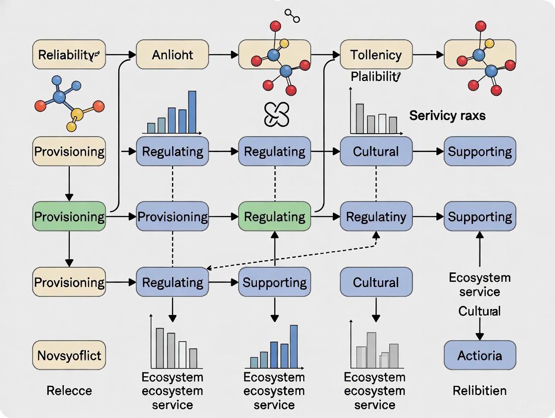
Q3: What are the standard categories for ecosystem services, and how are "benefits" classified within them?
A: Ecosystem services are typically broken down into four established categories [12] [13]. The "benefits" are the specific, often measurable, gains that humans receive from these services.
Table: Categories of Ecosystem Services and Their Associated Benefits
| Service Category | Description | Examples of Human Benefits |
|---|---|---|
| Provisioning | Material or energy outputs from ecosystems [12]. | Food, fresh water, raw materials (wood, fiber), genetic resources, and medicines [12] [13]. |
| Regulating | Benefits obtained from the moderation of ecosystem processes [12]. | Climate regulation, flood control, water purification, disease regulation, and pollination [12] [13]. |
| Cultural | Non-material benefits obtained from ecosystems [12]. | Recreational opportunities, aesthetic enjoyment, spiritual enrichment, and cognitive development [12] [13]. |
| Supporting | Services necessary for the production of all other ecosystem services [12]. | Soil formation, photosynthesis, nutrient cycling, and maintenance of genetic diversity [12] [13]. |
Q4: Our assessment model is yielding inconsistent results for cultural services. How can we improve reliability?
A: Challenges in quantifying cultural services are common, as they involve non-material, subjective benefits. To improve reliability:
- Employ mixed methods: Combine quantitative surveys and spatial analysis with qualitative techniques like interviews to capture both the physical access to and the perceived value of cultural spaces [15].
- Utilize the cascade framework: Ensure your study analyzes the full pathway from the ecosystem structure (e.g., a park) to the function (recreation) and its final impact on human well-being (e.g., improved mental health) [15].
- Expand scope: Studies focused solely on regulatory and supporting services should intentionally expand their scope to include the impact assessments of these services on human well-being, a step that is often missed [15].
Technical Troubleshooting Guide
This guide addresses common methodological issues encountered during integrated ecosystem service assessments.
Issue: Resolving Trade-offs and Synergies Between Multiple Ecosystem Services
Symptoms: Your model shows that enhancing one ecosystem service (e.g., food production through agriculture) leads to the decline of another (e.g., water purification or soil conservation). Conversely, you may find that some services are positively correlated [16].
Investigation & Resolution Protocol:
- Identify & Quantify: Use assessment tools like the InVEST model to quantitatively evaluate the individual services in question (e.g., water yield, carbon storage, habitat quality) over the same temporal and spatial scale [16].
- Correlation Analysis: Apply statistical methods to identify relationships. Common approaches include:
- Driver Analysis: Use machine learning regression models (e.g., Gradient Boosting Machines) to identify the key environmental and anthropogenic drivers influencing the observed trade-offs and synergies. This moves beyond correlation to identify potential causation [16].
- Scenario Planning: Project future land-use changes using models like the PLUS model under different scenarios (e.g., natural development, planning-oriented, ecological priority). Re-run your ecosystem service assessments for each scenario to inform planning decisions that optimize the desired suite of services [16].
Issue: Incorporating Spatial Dynamics and Scale into Assessments
Symptoms: The value or flow of an ecosystem service is not adequately captured, leading to inaccurate maps and conclusions about its availability to beneficiaries.
Investigation & Resolution Protocol:
- Define the Service-Providing Unit (SPU): Clearly map the ecosystem area that provides the service (e.g., a forest for carbon sequestration, a wetland for water filtration).
- Define the Service-Benefiting Area (SBA): Identify and map the location of the human populations or systems that benefit from the service (e.g., a downstream community for clean water).
- Model the Flow: Account for the spatial connectivity between the SPU and SBA. This can involve modeling the flow of water, movement of pollinators, or accessibility of recreational areas. Tools like the InVEST model and the RBI (Rapid Benefit Indicators) Approach can facilitate this spatial analysis [14] [16].
- Cross-Scale Analysis: Conduct analyses at multiple spatial scales (e.g., local, regional) to understand how the provision and demand for services change. This is particularly important for large cities and diverse regions [15].
Issue: Engaging Stakeholders and Capturing Value Plurality
Symptoms: Research outcomes are not adopted by policymakers or local communities, or the assessment fails to capture values that are not easily quantifiable in monetary terms.
Investigation & Resolution Protocol:
- Stakeholder Identification: Use structured tools like the FEGS (Final Ecosystem Goods and Services) Scoping Tool to identify and prioritize stakeholders and the specific environmental benefits they care about [14].
- Employ Non-Monetary Metrics: Utilize frameworks like the RBI (Rapid Benefit Indicators) Approach, which uses readily available data to estimate and quantify benefits to people using non-monetary indicators [14].
- Consider Alternative Frameworks: For culturally diverse contexts, consider using the Nature's Contributions to People (NCP) concept. This framework, developed by IPBES, can be more inclusive of worldviews beyond standard economic valuation [15].
Experimental Protocol for a Multi-Scenario ES Assessment
This protocol outlines a methodology for assessing ecosystem services under different future land-use scenarios, integrating machine learning for driver analysis.
Objective: To quantitatively assess and predict the dynamics of key ecosystem services, identify their drivers, and evaluate trade-offs under various future scenarios to inform regional ecological protection strategies [16].
Materials & Reagents:
Table: Key Research Reagent Solutions for ES Modeling
| Item | Function/Explanation |
|---|---|
| InVEST Model | A suite of open-source software models used to map and value the goods and services from nature that contribute to human well-being. It is central to quantifying specific services like carbon storage, water yield, and habitat quality [16]. |
| PLUS Model | A land-use simulation model used to project future changes in land use/cover under various scenarios. It excels at simulating complex dynamics at fine spatial scales [16]. |
| Machine Learning Library (e.g., scikit-learn) | Provides algorithms (e.g., Gradient Boosting) for identifying nonlinear relationships and key drivers within complex ecological datasets, improving predictive accuracy over traditional statistical methods [16]. |
| GIS Software (e.g., ArcGIS, QGIS) | A geographic information system for spatial data management, analysis, and the cartographic presentation of results. |
Methodology:
Data Acquisition & Harmonization:
- Collect spatial data for the study area, including: land use/cover maps, digital elevation models (DEMs), soil data, climate data (precipitation, temperature), and socio-economic data.
- Process all datasets to a consistent spatial resolution and projection to ensure comparability [16].
Historical ES Assessment:
- Use the InVEST model to quantify selected ecosystem services (e.g., water yield, carbon storage, habitat quality, soil conservation) for historical benchmark years (e.g., 2000, 2010, 2020).
- Calculate a comprehensive ecosystem service index to assess overall ecological capacity [16].
Driver Analysis with Machine Learning:
- Compile a dataset of potential driving factors (e.g., land use, vegetation index, precipitation, population density, GDP).
- Train and compare multiple machine learning models (e.g., Gradient Boosting, Random Forest) on the historical data to identify the most important drivers for each ecosystem service [16].
Future Scenario Design & Land Use Simulation:
- Design multiple future scenarios (e.g., 2035) reflecting different policy priorities:
- Natural Development Scenario: Projecting current trends.
- Planning-Oriented Scenario: Incorporating official development plans.
- Ecological Priority Scenario: Emphasizing conservation and restoration.
- Use the PLUS model, calibrated with historical data and informed by the driver analysis, to simulate land use changes for each scenario [16].
- Design multiple future scenarios (e.g., 2035) reflecting different policy priorities:
Future ES Assessment & Analysis:
- Run the InVEST model using the simulated land-use maps from Step 4 to evaluate ecosystem services under each future scenario.
- Analyze the trade-offs, synergies, and overall changes in ecosystem service capacity compared to the historical baseline [16].
Conceptual Diagram: The Ecosystem Service Cascade
The following diagram illustrates the logical progression from ecosystem structures to human well-being, as defined by the ecosystem service cascade framework.
Ecosystem services connect nature to human well-being.
Conceptual Diagram: Integrated ES Assessment Workflow
This diagram outlines the logical workflow for conducting an integrated ecosystem service assessment with multi-scenario prediction, as described in the experimental protocol.
Integrated workflow for ecosystem service assessment.
Troubleshooting Guides
Data Scarcity
Problem: Lack of locally relevant data for ecosystem service (ES) assessment at a regional scale.
- Solution: Employ a tiered approach for ES mapping. When data is scarce (Tier 1), use expert-based matrix approaches or simple GIS mapping with proxy indicators like land use/land cover (LULC) data to generate quick overviews [17]. Leverage citizen science-based data and knowledge co-generation to make the valuation process more inclusive and policy-oriented, filling critical data gaps at the local scale [18].
- Experimental Protocol: The expert-based ES matrix approach links ES values to appropriate geobiophysical spatial units, such as LULC types [17]. Values are classified on a relative scale (e.g., 0 to 5) to reduce complexity and allow comparisons between individual ES [17]. This protocol is cost-efficient and applicable in data-scarce areas [17].
Problem: Inability to use complex models due to data, time, or knowledge constraints.
- Solution: Use value transfer methods, where estimates of ES values per LULC from other published studies are applied to your area of interest [17]. While this provides a quick approximation, always explicitly state the sources and acknowledge the limitations of transferring data from a different context [17].
- Experimental Protocol: Compile a database of ES values from literature for various LULC classes. Apply these values to a regional LULC map using GIS software for spatial overlay. This generates a preliminary map of ES supply or value [19].
Conceptual Fuzziness
Problem: Ambiguity in defining and categorizing ecosystem services and their components.
- Solution: Adopt a generally accepted framework, such as the Common International Classification of Ecosystem Services (CICES), to reduce conceptual fuzziness and ensure a shared language [20]. Explicitly name the assessed ES components (e.g., potential supply, actual use, demand) in your assessment to avoid misinterpretations [20].
- Experimental Protocol: For transdisciplinary teams, implement a fuzzy set theory exercise. Have team members independently categorize system elements (e.g., a dam, forest management) as social, ecological, or technological, and then quantify their degree of membership (e.g., 50% social, 50% technological). This visually maps similarities and differences in perception, honoring diverse epistemological perspectives [21].
Problem: Conventional "crisp set" sustainability assessments make knife-edge conclusions that ignore inherent uncertainties.
- Solution: Implement a fuzzy logic approach for evaluation. This method uses fuzzy sets and conditional probabilities to assess sustainability, allowing for continuous gradations rather than sharp thresholds [22].
- Experimental Protocol:
- Define fuzzy sets for sustainability attributes (e.g., for income: "very low," "moderately low") [22].
- Develop fuzzy propositions about ecosystem sustainability (e.g., "biodiversity is moderately high") [22].
- Apply fuzzy logic rules to these propositions to reach a conclusion about the ecosystem's strong sustainability, which is more robust to uncertainty than crisp-set methods [22].
Spatial Heterogeneity
Problem: Understanding the complex spatial relationships and drivers of multiple ecosystem services.
- Solution: Analyze ES from an individual-pair-bundle perspective [23]. Quantify individual ES, statistically analyze trade-offs and synergies between ES pairs, and then use cluster analysis (e.g., K-means) to identify ES bundles—sets of services that repeatedly appear together in space [23] [24].
- Experimental Protocol:
- Map multiple key ES (e.g., water yield, carbon storage, habitat quality) using models or proxy data [23] [24].
- Use correlation analysis or spatial overlay to identify trade-offs (negative relationships) and synergies (positive relationships) between all ES pairs [23].
- Apply a clustering algorithm on the ES maps to delineate spatially explicit ES bundles. These bundles can then be used for targeted ecological function zoning [24].
Problem: Accounting for the flow of ecosystem services between service-producing areas and service-benefiting areas.
- Solution: Integrate supply-and-demand dynamics into valuation. Use a scarcity value model that adjusts the theoretical value of ES based on regional supply and socio-economic demand factors like population density and GDP [19].
- Experimental Protocol:
- Calculate the theoretical supply value of omni-directional and directional ES (e.g., gas regulation, water containment) [19].
- Adjust this value using demand factors (e.g., per capita GDP, population density) to calculate the ecosystem service scarcity value (ESSV) [19].
- Map the ESSV to reveal areas of high scarcity, which can serve as a reference for setting inter-regional ecological compensation prices [19].
Frequently Asked Questions (FAQs)
Q1: Does using an ecosystem services approach mean I have to put a dollar value on everything? A1: No. Using ecosystem services in decision-making does not require monetary valuation [25]. The value can be described in terms of health outcomes, material benefits, or through qualitative analyses that identify which services are most important to communities [25]. Monetary valuation is one useful tool among many for analyzing trade-offs [25].
Q2: How can I select the right mapping method for my specific research context? A2: Follow a tiered approach [17]. Let your research purpose, resources, and data availability guide you:
- Tier 1 (Rapid Assessment): For communication and awareness-raising. Use expert-based matrices, simple GIS with LULC proxies, or value transfer [17].
- Tier 2 (Intermediate Assessment): For more specific analysis. Use simple models (e.g., InVEST) or combine methods to assess a broader range of ES [17].
- Tier 3 (High-Resolution Assessment): For detailed, mechanistic understanding. Use complex, process-based models requiring high-quality, localized data [17].
Q3: We are a multidisciplinary team and can't agree on how to classify system elements. Is this a problem? A3: This is a common challenge and can be an opportunity. Different perspectives enrich the understanding of complex systems [21]. Instead of forcing a single classification, use a fuzzy SETS framework to acknowledge multiple memberships explicitly. This helps honor diverse epistemologies and creates a basis for deeper, more productive discussions about system dynamics [21].
Q4: What is the most common cause of unreliable ES assessment results? A4: A primary source of unreliability is the failure to explicitly recognize and address the underlying assumptions of the assessment [20]. These can range from conceptual and ethical foundations to assumptions about data representativeness, indicator validity, and economic rationality [20]. Increasing transparency about these assumptions and testing their consequences is crucial for improving reliability [20].
Quantitative Data Tables
Table 1: Ecosystem Service Scarcity Value (ESSV) Change in the Yangtze River Delta (2010-2020)
This table summarizes the impact of incorporating supply and demand dynamics on ecosystem service valuation, moving beyond theoretical value [19].
| Valuation Scenario | Total Value (2010) | Total Value (2020) | Percentage Change |
|---|---|---|---|
| Theoretical Value (ESTV) | Not Specified | Decreased by 8.67% | -8.67% |
| Scarcity Value (ESSV) | RMB 213 million | RMB 1.323 billion | +521.13% |
Table 2: Prevalence of Trade-offs and Synergies among Ecosystem Service Pairs
This table illustrates the complex relationships between ecosystem services, which is critical for understanding spatial heterogeneity. Data is illustrative of a study in Northeast China [23].
| Ecosystem Service | Relationship with Other ES | Percentage of ES Pairs Exhibiting Trade-offs |
|---|---|---|
| Carbon Storage (CS) | Trade-offs with over 70% of other ES | >70% |
| Habitat Quality (HQ) | Trade-offs with SC, WS, WP, AL | Not Specified |
| Overall ES Pairs | Synergies more prevalent than trade-offs | Less than 50% |
Methodological Workflows and Frameworks
Fuzzy Logic Assessment Workflow
ES Bundle Identification Workflow
Research Reagent Solutions
Table 3: Essential Data and Modeling Tools for ES Assessments
This table details key "research reagents"—data and tools essential for conducting integrated ES assessments.
| Item Name | Category | Primary Function | Key Considerations |
|---|---|---|---|
| Land Use/Land Cover (LULC) Data | Spatial Data | Serves as a fundamental proxy for mapping the potential supply of many ES (e.g., food, carbon storage) [17]. | Widely accessible (e.g., Urban Atlas); may not capture ecological quality or management intensity [17]. |
| InVEST Models | Software Tool | A suite of open-source, spatially explicit models for quantifying and valuing multiple ES (e.g., carbon storage, water yield) [17]. | Requires intermediate GIS skills; each model has specific data input requirements [17]. |
| Expert-Based ES Matrix | Methodology | A lookup table that assigns ES scores to LULC classes, enabling rapid ES assessment in data-scarce contexts [17]. | Subjectivity requires careful expert selection; best for communication and initial screening [20] [17]. |
| Multiscale Geographically Weighted Regression (MGWR) | Statistical Tool | Analyzes spatial non-stationarity and identifies driving factors of ES patterns across a landscape [23]. | Reveals how the influence of drivers (e.g., slope, GDP) varies across space, explaining heterogeneity [23]. |
Advanced Tools and Techniques for Integrated ES Assessment
Troubleshooting Guides & FAQs
InVEST Model Troubleshooting
Q: My InVEST model runs but produces illogical results (e.g., negative water yield values). What should I check?
A: This commonly stems from input data issues. Please verify the following:
- Data Format and Projection: Ensure all input raster and vector files are in the same, supported coordinate reference system (CRS). InVEST requires projected CRS (e.g., UTM) rather than geographic coordinates (e.g., WGS84) for accurate area and distance calculations [26].
- Input Data Validity: Check that all input rasters (e.g., Land Use/Land Cover (LULC), DEM) contain valid, positive values where expected. Search for and replace NoData values or negative numbers that are not biologically meaningful [27].
- Preprocessing with Helper Tools: Use InVEST's built-in helper tools like
RouteDEMfor advanced flow direction and accumulation calculations, which can improve the hydrological inputs for models like the Annual Water Yield [28].
Q: How can I visualize and share my InVEST results more effectively?
A: Beyond traditional GIS, the InVEST team offers two powerful solutions:
- InVEST Dashboards: This feature allows you to create interactive, web-based visualizations of your results. You can explore outputs with interactive maps and charts and share them with colleagues via a simple link, eliminating the need for complex GIS symbology [28].
- Python API: For advanced users, the InVEST Python API enables integration into custom scripts and complex analytical workflows, allowing for automated post-processing and visualization [28].
Q: What is the difference between the "classic" InVEST application and the new "Workbench"?
A: The InVEST Workbench is a repackaged version of the same InVEST models with a new user interface. It provides all the same functionality with the goal of being more accessible and extensible. The classic application remains available, but the Workbench represents the future of the software [26].
PLUS Model Troubleshooting
Q: My PLUS model simulation fails to start or crashes during the Land Expansion Analysis Strategy (LEAS) phase. What could be the cause?
A: This is often related to input data format or system compatibility.
- Data Format Compatibility: Ensure all your input raster data (e.g., LULC maps, driving factor maps) have the same spatial extent, cell size, and coordinate system. Mismatches are a frequent cause of failure [29].
- Software Environment: Confirm that you have the correct version of the PLUS model for your operating system and that all necessary dependencies (like specific .NET Framework versions) are installed. Consult the user manual for specific system requirements [29].
Q: The simulated land use pattern from PLUS appears highly fragmented and unrealistic. How can I improve it?
A: You can adjust the model's parameters to better reflect real-world land use dynamics:
- CAAF Module Parameters: Tune the parameters within the Cellular Automata (CA) model, specifically the neighborhood weight and conversion cost matrix. These settings control the influence of surrounding land use types and the ease with which one land type can convert to another. Refer to the user manual for detailed guidance on these parameters [29].
RUSLE Model Integration Troubleshooting
Q: When integrating RUSLE with InVEST for a comprehensive ecosystem service assessment, how should I handle discrepancies in spatial resolution between models?
A: Consistency is key for integrated assessments.
- Resample to a Common Resolution: Choose a target spatial resolution that is appropriate for your study area and research question. All input layers for both RUSLE (e.g., rainfall erosivity, soil erodibility) and InVEST (e.g., LULC for the Sediment Delivery Ratio model) should be resampled to this identical resolution and extent [27]. This ensures that the outputs from one model can be correctly used as inputs for another.
Q: What is the best way to validate the soil conservation results from an integrated InVEST-RUSLE analysis?
A: A multi-faceted validation approach is recommended [27]:
- Field Measurements: Compare your modeled soil retention values with empirical data from sediment traps or erosion pins in the field, if available.
- Spatial Pattern Checks: Visually compare the spatial pattern of predicted soil erosion with high-resolution imagery or known erosion features (e.g., gullies) to assess if the model captures "hotspots" correctly.
- Literature Comparison: Benchmark your results against soil erosion rates reported in scientific literature for similar regions and land cover types.
Table 1: Key Ecosystem Services and Corresponding Models for Integrated Assessment.
| Ecosystem Service | Primary Model | Quantifiable Outputs | Key Input Data Requirements |
|---|---|---|---|
| Water Yield | InVEST | Water yield volume (mm) | LULC, DEM, precipitation, soil depth, plant available water content [27] |
| Carbon Storage | InVEST | Carbon storage (tons) in four pools | LULC, carbon pool data (above/biomass, belowground, soil, dead organic matter) [27] |
| Habitat Quality | InVEST | Habitat quality/degradation index (0-1) | LULC, threat data sources (e.g., roads, urban areas), threat sensitivity [27] |
| Soil Conservation | InVEST / RUSLE | Soil retention (tons/ha) | Rainfall erosivity (R), soil erodibility (K), DEM, LULC, management factor (C & P) [27] |
| Land Use Simulation | PLUS | Future land use maps, transition probabilities | Historical LULC maps, driving factors (e.g., slope, population), development constraints [29] |
Table 2: Summary of a Recent Integrated Assessment Study Using InVEST and RUSLE (Central Yunnan Province, 2000-2020) [27].
| Ecosystem Service | Trend (2000-2020) | Primary Drivers (q-value rank) | Notes |
|---|---|---|---|
| Water Yield (WY) | Increasing | Relief degree of land surface (RDLS), Slope, NDVI | Modeled using InVEST |
| Carbon Storage (CS) | Decreasing | Relief degree of land surface (RDLS), Slope, NDVI | Modeled using InVEST |
| Habitat Quality (HQ) | Increasing | Relief degree of land surface (RDLS), Slope, NDVI | Modeled using InVEST |
| Soil Conservation (SC) | Increasing | Relief degree of land surface (RDLS), Slope, NDVI | Modeled using RUSLE |
| Integrated Index (IESI) | Decreased then Increased | Analysis via Optimal Parameter-based Geographical Detector (OPGD) | Constructed using Principal Component Analysis (PCA); Optimal detection scale was 4500m grid. |
Experimental Protocols for Integrated Assessment
Protocol: Spatio-Temporal Assessment of Multiple Ecosystem Services
This protocol is derived from a 2025 study that integrated InVEST and RUSLE to evaluate ecosystem services in Central Yunnan Province (CYP) [27].
1. Study Area Definition:
- Clearly delineate the spatial boundary of the study area (e.g., CYP: 94,558 km²).
- Document the key characteristics of the area, such as dominant landforms, climate, and prevailing socio-economic activities.
2. Data Collection and Preprocessing:
- Gather time-series data for the study period (e.g., 2000, 2005, 2010, 2015, 2020).
- Core data includes: LULC maps, Digital Elevation Models (DEMs), meteorological data (precipitation, temperature), soil type maps, and socio-economic data if needed.
- Crucially, preprocess all spatial data to a common coordinate system, spatial extent, and cell size.
3. Ecosystem Service Modeling:
- Run InVEST Models: Execute the relevant InVEST models (e.g., Annual Water Yield, Carbon Storage, Sediment Delivery Ratio, Habitat Quality) for each time point using the preprocessed data [27].
- Run RUSLE Model: Calculate soil conservation service using the Revised Universal Soil Loss Equation, which estimates potential soil loss without vegetation minus the actual soil loss [27].
4. Data Integration and Index Construction:
- Normalize the outputs of the four key services (WY, CS, HQ, SC) to make them comparable.
- Use Principal Component Analysis (PCA) to construct an Integrated Ecosystem Service Index (IESI). This method objectively determines the weight of each service based on its contribution to the overall variance, avoiding subjective weighting [27].
5. Driving Force Analysis:
- Select potential driving factors (e.g., RDLS, slope, NDVI, population density, precipitation).
- Use the Optimal Parameter-based Geographical Detector (OPGD) model to identify the key drivers and their interaction effects on the spatial divergence of ecosystem services. This method helps determine the optimal spatial scale for analysis [27].
Protocol: Scenario Analysis with Land Use Projection
1. Historical Land Use Change Analysis:
- Use two historical LULC maps (e.g., from 2000 and 2010) to analyze transitions and develop transition probability matrices.
2. Land Use Simulation with PLUS:
- Utilize the PLUS model, which combines the Land Expansion Analysis Strategy (LEAS) and a Cellular Automata (CA) model with a Patch-generating Simulation (CARS) mechanism.
- Input historical LULC and driving factors into the LEAS module to extract land expansion patterns and transition probabilities.
- Simulate future LULC (e.g., for 2020) using the CA model. Validate the simulation by comparing it to the actual 2020 LULC map [29].
3. Future Ecosystem Service Assessment:
- Use the simulated future LULC map from PLUS as a primary input for the InVEST and RUSLE models.
- Run the ecosystem service models under the simulated future scenario to assess the potential impact of land use change on service provision.
Workflow Visualization
Integrated Ecosystem Services Assessment Workflow
Research Reagent Solutions: Essential Data & Tools
Table 3: Essential "Research Reagents" for Integrated Spatial Modeling.
| Item / Tool | Type | Primary Function in Analysis |
|---|---|---|
| LULC Maps | Core Input Data | The foundational layer representing earth's surface; primary driver for estimating service supply (e.g., carbon, habitat) in InVEST and for change analysis in PLUS [27]. |
| Digital Elevation Model (DEM) | Core Input Data | Used for calculating slope, flow direction, and watershed delineation; critical for hydrological modeling in InVEST and RUSLE, and as a driving factor in PLUS [28] [27]. |
| InVEST Helper Tools (RouteDEM, DelineateIT) | Preprocessing Tool | Enhances input data quality. RouteDEM calculates advanced flow routing, while DelineateIT automates watershed delineation, improving inputs for freshwater models [28]. |
| RUSLE Factors (R, K, C, P) | Model Parameters | The core components for calculating soil loss: Rainfall Erosivity (R), Soil Erodibility (K), Cover Management (C), and Support Practice (P) [27]. |
| Principal Component Analysis (PCA) | Statistical Method | Used to objectively integrate multiple ecosystem service metrics into a single, comprehensive index (IESI), avoiding subjective weighting [27]. |
| Optimal Parameter-based Geographical Detector (OPGD) | Analysis Tool | Identifies the key driving factors behind the spatial patterns of ecosystem services and determines the optimal scale for analysis [27]. |
Frequently Asked Questions (FAQs)
FAQ 1: What is the most objective method to assign weights when constructing an IESI? Principal Component Analysis (PCA) is a highly objective method for constructing an IESI. Unlike cumulative equations, maximum value methods, or subjective weighting approaches like the Analytic Hierarchy Process (AHP), PCA uses the data structure itself to determine weights. It reduces dimensionality while concentrating information, objectively considering the relative importance of multiple ecosystem service indicators without researcher bias [27].
FAQ 2: Which ecosystem services should I include in my IESI? The specific services depend on your regional context, but commonly assessed key services include Water Yield (WY), Carbon Storage (CS), Habitat Quality (HQ), and Soil Conservation (SC). These represent crucial provisioning, regulating, and supporting services. In the Central Yunnan Province case study, these four services provided a comprehensive foundation for integration [27].
FAQ 3: My IESI shows a decreasing trend. What are the most likely causes? A declining IESI often reflects landscape degradation. Key drivers to investigate include:
- Land Use/Cover Change (LUCC), particularly conversion of natural areas to agriculture or urban use
- Changes in vegetation cover (declining NDVI)
- Topographic factors like relief degree of land surface (RDLS) and slope
- Climate factors affecting ecosystem processes [27]
FAQ 4: What is the optimal spatial scale for analyzing driving forces behind my IESI? The optimal scale varies by region. In Central Yunnan Province, a 4500 m × 4500 m grid was identified as optimal for detecting the spatial divergence of comprehensive ecosystem services using the OPGD model. You should test multiple scales in your study area, as key driving factors may shift with changing spatial scales [27].
FAQ 5: How can I validate my IESI results? Validation can be achieved through:
- Comparing spatio-temporal trends against known environmental changes
- Testing the IESI's response to documented policy implementations
- Analyzing driving mechanisms using geographical detector models
- Correlating with independent environmental quality indicators [27]
Troubleshooting Guides
Problem 1: Subjectivity in Weighting Multiple Ecosystem Services
Symptoms: Difficulty justifying weight assignments; results vary significantly with different weighting schemes.
Solution: Implement Principal Component Analysis (PCA)
- Standardize all ecosystem service datasets to ensure comparability
- Run PCA on the correlation matrix of your ecosystem services
- Extract weights from the first principal component loadings
- Calculate IESI using the formula: IESI = Σ(Standardized ES value × PCA-derived weight)
- Verify that the first principal component explains sufficient variance (>70% is ideal) [27]
Problem 2: Inconsistent Spatial Scales Causing Integration Issues
Symptoms: Data misalignment; artifacts at boundaries; difficulty interpreting results.
Solution: Establish Consistent Spatial Framework
- Identify optimal analysis scale using the OPGD model at multiple grid sizes
- Resample all data to common resolution and extent before integration
- Validate scale choice by ensuring key drivers maintain explanatory power
- Document all scale transformations for reproducibility [27]
Problem 3: Handling Conflicting Trends in Individual Ecosystem Services
Symptoms: Some services improve while others degrade; unclear overall ecosystem status.
Solution: Implement Trend Analysis and Trade-off Identification
- Calculate temporal trends for each service individually using linear regression
- Identify trade-offs and synergies through correlation analysis
- Interpret IESI in context of individual service trajectories
- Report both integrated and disaggregated results for comprehensive understanding [27]
Experimental Protocols and Data
Protocol 1: IESI Construction via Principal Component Analysis
Purpose: To objectively integrate multiple ecosystem services into a single composite index.
Materials:
- Spatially explicit datasets for target ecosystem services
- GIS software with raster calculation capabilities
- Statistical software with PCA functionality
Procedure:
- Data Preparation: Standardize each ecosystem service layer to zero mean and unit variance
- Spatial Alignment: Ensure all layers share identical projection, extent, and cell size
- PCA Execution: Extract principal components from the correlation matrix
- Weight Assignment: Use first principal component loadings as integration weights
- Index Calculation: Compute weighted sum: IESI = w₁×ES₁ + w₂×ES₂ + ... + wₙ×ESₙ
- Validation: Check that first component explains sufficient variance (>50%) [27]
Protocol 2: Driving Force Analysis using OPGD Model
Purpose: To identify key factors influencing IESI spatial patterns.
Materials:
- IESI spatial distribution data
- Candidate driving factor datasets (topography, climate, vegetation, human activity)
- Optimal parameter-based geographical detector (OPGD) software
Procedure:
- Factor Selection: Compile potential driving factors based on ecological relevance
- Scale Optimization: Test multiple spatial scales to identify optimal detection scale
- Factor Detection: Calculate q-values for each factor using geographical detector
- Interpretation: Rank factors by explanatory power (q-value)
- Interaction Analysis: Test factor interactions for enhanced understanding [27]
Table 1: IESI Values in Central Yunnan Province (2000-2020) [27]
| Year | Mean IESI Value | Trend Direction | Key Influencing Factors |
|---|---|---|---|
| 2000 | 0.7338 | Baseline | RDLS, Slope, NDVI |
| 2005 | 0.6981 | Decreasing | Land use change, vegetation cover |
| 2010 | 0.6947 | Stable | Climate factors, topography |
| 2015 | 0.6650 | Decreasing | Human activity intensity |
| 2020 | 0.6992 | Increasing | Conservation policies, management |
Table 2: Ecosystem Service Assessment Methods [27]
| Ecosystem Service | Assessment Model | Key Inputs | Output Metrics |
|---|---|---|---|
| Water Yield (WY) | InVEST | Precipitation, evapotranspiration, soil depth | mm/year |
| Carbon Storage (CS) | InVEST | Land use, carbon pools (above, below, soil, dead) | Mg/ha |
| Habitat Quality (HQ) | InVEST | Land use, threat sources, sensitivity | 0-1 index |
| Soil Conservation (SC) | RUSLE | Rainfall, soil erodibility, topography | t/ha/year |
The Scientist's Toolkit
Table 3: Essential Research Reagents and Computational Tools
| Tool/Reagent | Function | Application in IESI Research |
|---|---|---|
| InVEST Model Suite | Spatially explicit ecosystem service modeling | Quantifying water yield, carbon storage, habitat quality |
| RUSLE Model | Soil erosion estimation | Calculating soil conservation service |
| Geographical Detector | Spatial stratified heterogeneity analysis | Identifying driving forces behind IESI patterns |
| Principal Component Analysis | Multivariate data reduction | Objectively weighting and integrating multiple ES |
| Normalized Difference Vegetation Index | Vegetation vigor assessment | Serving as proxy for ecosystem productivity |
Workflow Visualization
IESI Construction and Analysis Workflow
Ecosystem Service Integration Methodology
Harnessing Machine Learning and Geodetector Models for Driver Analysis
Frequently Asked Questions (FAQs)
FAQ 1: What is the fundamental difference between driver analysis and Geodetector?
Driver analysis typically refers to a set of statistical methods, often based on regression, used to estimate the importance of various independent variables (drivers) in predicting a dependent variable. For example, it can use Linear Regression Coefficients, Shapley Regression, or Relative Importance Analysis to compute importance scores [30]. In contrast, Geodetector is a specialized tool designed to measure and attribute spatially stratified heterogeneity (SSH). Its core function is to test the coupling between two variables (Y and X) without assuming linearity and to investigate interactions between explanatory variables [31].
FAQ 2: My Geodetector model fails to run. What are the most common data requirements I should check?
The most common data requirements for Geodetector that can cause runtime failures are:
- Variable Types: The response variable (Y) must be numerical. The explanatory factors (X) must be categorical (e.g., landuse types, seasons). If your X variables are numerical, you must first discretize them into strata [32].
- Sample Size: The data must contain a sufficient number of samples. There should be at least three sample units within each stratum of a factor [32].
- Data Volume: While not specific to Geodetector, related analytical platforms often enforce data volume limits (e.g., a maximum file size of 40 MB), which is a good general checkpoint [33].
FAQ 3: Why does my machine learning model have poor performance even after using driver analysis for feature selection?
Poor model performance can stem from issues beyond feature importance. Common culprits include:
- Implementation Bugs: Incorrect tensor shapes, improper loss function inputs, or errors in toggling between training and evaluation modes can cause silent failures [34].
- Data-Model Fit: The model architecture might be too simple or too complex for your data. It is recommended to start with a simple architecture (e.g., a fully-connected network with one hidden layer, or a LeNet for images) and sensible hyper-parameter defaults [34].
- Data Quality: The problem could be in the dataset itself, such as noisy labels, imbalanced classes, or a mismatch between the training and test set distributions [34] [35].
FAQ 4: What should I do if my driver analysis results seem counter-intuitive or unreliable?
First, always remember that driver analysis offers insights to aid decision-making but does not guarantee absolute accuracy. Correlation does not imply causation [33].
- Check for Correlated Predictors: If your independent variables are highly correlated, methods like Linear Regression Coefficients can become unreliable. In such cases, switch to methods designed to handle multicollinearity, such as Shapley Regression or Relative Importance Analysis [30] [36].
- Review Diagnostics: Ensure you have reviewed technical diagnostics for outliers and heteroscedasticity. Also, check the p-values and standard errors of the importance scores to assess their statistical significance [36].
- Validate with a Simple Baseline: Compare your model's performance against a simple baseline (e.g., the average of outputs or a linear regression) to verify that it is learning meaningful patterns [34].
Troubleshooting Guides
Issue 1: Preparing and Integrating Data for Combined ML and Geodetector Workflows
Problem: Users are unsure how to structure their data and preprocess variables to be compatible with both machine learning and Geodetector models.
Solution: Follow this integrated data preparation protocol.
Step 1: Variable Transformation and Discretization Geodetector requires categorical X variables. You must discretize any continuous explanatory variables.
- Methodology: For a continuous variable (e.g., "GDP per capita" or "elevation"), stratify the values into a discrete number of meaningful strata (e.g., 5 strata: Very Low, Low, Medium, High, Very High) [32]. The boundaries can be defined using natural breaks, quantiles, or domain knowledge.
- Integration Note: The same discretized variables can then be used as features in your machine learning model, often by converting them into one-hot encoded representations.
Step 2: Data Formatting
- Geodetector Format: For the Excel version of Geodetector, data should be formatted with each row representing a sample unit (e.g., a village). The first column is the numerical response variable (Y), and subsequent columns are the categorical factors (X) [32].
- ML Format: Ensure the dataset is split into training and testing sets. Normalize the input data for the ML model by subtracting the mean and dividing by the standard deviation. For images, it is sufficient to scale values to [0, 1] [34].
Step 3: Data Volume and Quality Check
Issue 2: Selecting the Appropriate Driver Analysis Method
Problem: With multiple driver analysis methods available, users often select an inappropriate one, leading to misleading results, especially with correlated predictors.
Solution: Select a method based on the characteristics of your predictors and your research goal. The table below summarizes the key methods.
Table 1: Comparison of Driver Analysis Methods
| Method | Core Principle | Best Used When | Key Consideration |
|---|---|---|---|
| Linear Regression Coefficients [30] | Normalized absolute values of regression coefficients. | You need to understand the sensitivity of Y to changes in X, and predictors are independent. | Highly unreliable when predictors are correlated. |
| Contribution [30] | Explains variance based on both the coefficient and the variation in the data. | You want to measure the historical impact of variables, not just their potential. | Is scale-independent. |
| Shapley Regression [30] [36] | Averages the incremental R² improvement across all possible variable orderings. | Predictors are correlated, and you need a robust measure of importance. | Computationally intensive for >15 variables; may auto-switch to Relative Importance Analysis. |
| Relative Importance Analysis [30] | Uses orthogonalized predictors to disentangle correlated contributions. | You have many correlated predictors (>15) and need a faster alternative to Shapley. | Provides results highly similar to Shapley but is computationally more efficient. |
The following workflow can help visualize the selection process:
Issue 3: Debugging and Improving a Machine Learning Model
Problem: A model has been implemented, but its performance is low, and the cause is unknown.
Solution: Adopt a systematic troubleshooting strategy.
Step 1: Start Simple The key is to start simple and gradually ramp up complexity [34].
- Architecture: Choose a simple architecture (e.g., a fully-connected network with one hidden layer, LSTM with one layer for sequences, LeNet for images).
- Defaults: Use sensible defaults: ReLU activation, no regularization, and normalized inputs.
- Problem: Simplify the problem by working with a small training set (e.g., ~10,000 examples) or a synthetic dataset to ensure the model can learn at all.
Step 2: Implement and Debug
- Overfit a Single Batch: The most critical heuristic. Try to drive the training error on a single batch of data arbitrarily close to zero. This catches a vast number of bugs [34].
- If the error explodes, it is often a numerical issue or a learning rate that is too high.
- If the error oscillates, lower the learning rate and inspect the data.
- If the error plateaus, increase the learning rate and inspect the loss function and data pipeline.
- Common Bugs: Check for incorrect tensor shapes, improper input preprocessing (e.g., forgetting to normalize), and incorrect input to the loss function [34].
- Overfit a Single Batch: The most critical heuristic. Try to drive the training error on a single batch of data arbitrarily close to zero. This catches a vast number of bugs [34].
Step 3: Evaluate and Analyze Errors
- Bias-Variance: Apply bias-variance decomposition to prioritize the next steps [34].
- Error Analysis: Create a dataset with target values, predictions, and prediction probabilities. For categorical features, group by each category and calculate the mean accuracy. This helps identify specific categories (e.g., "Month-to-month" contract type) or value ranges where the model performs poorly [35].
The following diagram outlines a high-level debugging decision tree:
Table 2: Key Software and Analytical Tools for Integrated Driver Analysis
| Item | Function | Relevance to Research |
|---|---|---|
| Geodetector Software [31] [32] | A statistical tool to measure spatially stratified heterogeneity and detect interactions between factors. | Core tool for analyzing the driving forces behind spatial patterns in ecosystem services without assuming linearity. |
| Shapley Regression [30] [36] | A driver analysis method that robustly handles correlated predictors by averaging over all possible models. | Provides reliable variable importance scores when ecological predictors are collinear (e.g., elevation, soil type, precipitation). |
| Relative Importance Analysis [30] | A computationally efficient alternative to Shapley for datasets with a large number of predictors. | Essential for analyzing high-dimensional datasets, such as those incorporating numerous remote sensing indices or climate variables. |
| LightGBM Classifier [35] | A high-performance gradient boosting framework based on decision tree algorithms. | A powerful machine learning model for classification and regression tasks in ecosystem prediction, such as modeling land use change or species distribution. |
| Optuna [35] | A hyperparameter optimization framework for automating the search for the best model parameters. | Crucial for systematically tuning machine learning models to achieve peak predictive performance on ecosystem service data. |
Frequently Asked Questions (FAQs) for Researchers
This section addresses common conceptual and practical questions researchers encounter when integrating local knowledge into ecosystem services assessments.
Table 1: Frequently Asked Questions on Citizen Science and Participatory Mapping
| Question | Answer & Application to Ecosystem Services Research |
|---|---|
| What is local knowledge and why is it valuable for ecosystem services (ES) research? | Local knowledge is a place-based, experiential system of knowledge developed by people who depend upon an ecosystem [37]. Unlike siloed scientific data, it communicates connections in social-ecological systems, providing fine-scale, spatially explicit data that can fill critical information gaps in ES appraisals, thereby enhancing their reliability [37] [38]. |
| How can local knowledge improve the reliability of ES assessments? | It provides fine-scale data on system change, informs locally relevant hypotheses, and captures social and ecological data in tandem [37]. This helps address information gaps and cumulative uncertainties in governance-relevant ES appraisals, moving beyond potential service values to understanding actual benefits accrued by society [38] [39]. |
| What is the "right to research" in this context? | Coined by Arjun Appadurai, it is the concept that the capacity to perform systematic inquiry is a right and a crucial tool for all citizens. In ES research, this means empowering local communities to document their knowledge and use it to intervene in issues that affect their lives, fostering a more democratic and relevant science [40]. |
| What are the main participatory mapping methods? | Participatory Mapping: Engages participants to map ES, locate conflicts, and highlight threatened areas, often using tools like PGIS [41]. Photovoice: Allows participants to use photography to highlight local issues and aspects of their life associated with ES, providing qualitative context [41]. |
| What is a key challenge in integrated ES appraisals? | An "information gap" can exist where the decision context requires high accuracy and reliability, but the expected uncertainty of ES appraisal methods is also high, making their use less likely. Participatory methods can help bridge this gap by providing missing local context [38]. |
Troubleshooting Guides for Experimental Protocols
This section provides step-by-step solutions for common methodological challenges.
Troubleshooting Guide 1: Overcoming Lack of Community Participation
Problem: Difficulty in recruiting or sustaining engagement from local community members in your participatory mapping project.
Root Cause: This often stems from a lack of community buy-in, persistent power structures that prioritize expert knowledge, or a research design that does not address locally identified problems [37].
Solutions:
- Employ a Co-Production Model: Frame the project from the bottom-up, focusing on collaborative inquiry and developing solutions to community-identified problems. Researchers should act as facilitators [37].
- Ensure Equitable Exchange: Design the process so that the community gains immediately valuable knowledge, capacity, or tools from participation, reinforcing their "capacity to aspire" [40].
- Utilize Appropriate Tools: For communities with lower literacy, combine methods like Photovoice and group discussions to ensure diverse participation and anonymous input [41].
The following workflow outlines a co-production approach to ensure meaningful community participation from start to finish:
Problem: How to systematically combine qualitative local knowledge with quantitative scientific data for a robust ES assessment.
Root Cause: Local knowledge and scientific data often differ in scale, format, and epistemology, creating integration challenges [38] [39].
Solutions:
- Adopt a Structured Framework: Use a tailored social-ecological systems (SES) framework to guide the accumulation and synthesis of social and ecological variables [37].
- Use Participatory Mapping as a Bridge: Spatial data from mapping can be directly incorporated into Geographic Information Systems (GIS) to enrich technical spatial analyses [41] [40].
- Leverage Integrated Modeling Methodologies: Employ approaches like the ARIES methodology, which uses artificial intelligence to assist in assembling customized models that can handle diverse data types and explicitly quantify uncertainty [39].
Table 2: Research Reagent Solutions for Participatory Mapping
| Research 'Reagent' | Function in Experimental Protocol |
|---|---|
| Social-Ecological Systems (SES) Framework | A conceptual scaffold to identify and organize key variables and relationships between resource systems, governance, users, and resource units, ensuring all relevant factors are considered [37]. |
| Participatory GIS (PGIS) | A technological tool that integrates local spatial knowledge from participants into a digital mapping environment, creating visually compelling and analytically robust data layers [40]. |
| Photovoice Methodology | A qualitative method that provides context and meaning to spatial data. It allows community members to document and discuss their realities through photography, highlighting issues unknown to outsiders [41]. |
| Semi-Structured Interviews | A data collection technique used alongside participatory mapping to gather in-depth qualitative data that explains and enriches the mapped information, providing the "why" behind the "where" [37]. |
Detailed Experimental Protocols from Cited Studies
This section provides reproducible methodologies from key studies.
Protocol 1: Participatory Mapping for Coastal Marine SES (Maine, USA)
This protocol demonstrates how to co-produce fine-scale data on a social-ecological system [37].
- Objective: To document local knowledge of coastal marine systems to inform collaborative research on changes in shellfish species, predators, and human activities.
- Theoretical Framework: The research is guided by a social-ecological system (SES) framework tailored for benthic small-scale fisheries [37].
- Methodology:
- Participatory Mapping: Conduct mapping sessions with local resource users (e.g., shellfish harvesters) to spatially document their knowledge of the system.
- Semi-Structured Interviews: Perform interviews alongside mapping to gather detailed contextual information.
- Data Integration: Synthesize mapped spatial data and interview transcripts to characterize the SES, generate local hypotheses, and directly inform the design of subsequent ecological research projects [37].
Protocol 2: Integrating Participatory Mapping and Photovoice (Tun Mustapha Park, Malaysia)
This protocol combines two participatory methods to elicit a comprehensive understanding of ecosystem services [41].
- Objective: To understand ecosystem services, their dynamics, and the anthropogenic impacts on marine-associated habitats from the community perspective.
- Methodology:
- Participatory Mapping: Invite participants from community-based organizations to map the location of ecosystem services.
- Photovoice: Equip participants with cameras to document ecological, sociocultural, and economic issues surrounding the ecosystem services.
- Group Discussions: Facilitate discussions about the maps and photographs, allowing participants to provide in-depth qualitative data, highlight issues, and develop consensus views and recommendations [41].
- Output: The process generates rich visual, spatial, and qualitative data to enhance ecosystem-based management and empowers participants to engage in governance [41].
The following diagram illustrates the logical flow of this integrated methodology, showing how different components connect to produce scientific and community outcomes:
Navigating Pitfalls and Optimizing ES Assessment Practices
Identifying and Mitigating Prevalent Assumptions in ES Modeling
Frequently Asked Questions
What are assumptions in the context of Ecosystem Services (ES) modeling? Assumptions are implicit or explicit statements that are accepted as true without immediate proof. They are necessary to simplify the immense complexity of real-world social-ecological systems, making ES assessments manageable. However, if they are ambiguous or inappropriate, they can lead to misconceptions and reduce the usefulness of the assessment for conservation decisions [20].
Why is it critical to identify assumptions in my model? Unchecked assumptions are a primary source of Requirements Technical Debt (RTD). If these assumptions are incomplete, incorrect, or become invalid over time, they can lead to system failures, unexpected behavior, and costly rework much later in the project lifecycle. Explicitly managing assumptions is fundamental to improving the reliability and dependability of your research outcomes [42].
My ES model is producing unrealistic results. Where should I start troubleshooting? Begin by isolating the section of the model or the specific geoprocessing tool that is causing the error. Run the tool outside the model with the same inputs to see if the issue persists. This helps determine if the problem is with the tool itself, the model structure, or the data inputs [43]. Furthermore, validate your model against independent population or field data if available; a model's ability to recreate multiple observed patterns in real data is a strong indicator that its assumptions and structure are appropriate [44].
Are there standardized tools for managing environmental assumptions? While there is no single universal standard, several modeling frameworks provide structured support. A comparative evaluation of representative approaches shows that KAOS and Obstacle Analysis are particularly strong for explicitly modeling assumptions and their potential violations. SysML excels at integration with broader systems engineering workflows, and RDAL demonstrates superior capabilities in tracing the relationships between assumptions, requirements, and verification conditions [42].
A common assumption is that my data are representative. What if they are not? Using secondary data or data from a different spatial or temporal context can severely limit the credibility of your assessment when applied to a specific area, like a protected area. To mitigate this, ask local communities for their knowledge, use adjusted value-transfer functions, and always collect field data to evaluate uncertainties in the transferred data [20].
Troubleshooting Guides
Issue 1: Unrealistic or Highly Uncertain Model Outputs
This often stems from foundational assumptions about the system that do not hold true.
Potential Cause 1: Over-simplification of ecological complexity. Your model may treat ecosystem services as independent entities, ignoring critical synergies and trade-offs [20].
- Mitigation Strategy:
- Move beyond quantifying individual services and study their interactions over time and space [20].
- Employ functional trait-based models to better capture the ecological mechanisms that underpin multiple services [20].
- Use scenario analysis to predict how changes in land use or climate will affect the bundle of services [45].
- Mitigation Strategy:
Potential Cause 2: Invalid indicator. The proxy you are using to represent the ecosystem service may not be a credible measure of the service itself, neglecting key ecological relationships [20].
Potential Cause 3: Violated model structure assumptions. Your population projection model may rely on common assumptions, such as a 1:1 offspring sex ratio, density-independent vital rates, or a demographically closed population, which may be inappropriate for your species [44].
- Mitigation Strategy:
Table 1: Common Assumptions in Population Projection Models and Their Conservation Relevance
| Assumption | Description | Potential Impact on Conservation Inference |
|---|---|---|
| Closed Population | No immigration or emigration. | Can severely overestimate or underestimate extinction risk for populations with source-sink dynamics or in fragmented landscapes [44]. |
| Female-Only Dynamics | Model includes only females, assuming males are not limiting. | May underestimate extinction risk if mate availability is a limiting factor or in small populations [44]. |
| Density Independence | Vital rates (birth, death) do not change with population size. | Can misrepresent population growth, especially near carrying capacity, and lead to incorrect predictions about recovery [44]. |
| Constant Vital Rates | Vital rates do not vary over time. | Ignores the impact of environmental stochasticity (e.g., good/bad years), leading to overconfident and potentially inaccurate projections [44]. |
| Uncorrelated Rates | Vital rates are statistically independent. | If rates are correlated (e.g., a bad year lowers birth rate and raises death rate), it increases extinction risk, which this assumption would overlook [44]. |
Issue 2: Model Results Are Rejected or Misinterpreted by Stakeholders
This can occur due to mismatches between the model's conceptual foundation and the stakeholders' values or understanding.
Potential Cause 1: Implicit worldview and ethical preconceptions. The ES model, by its nature, emphasizes anthropocentric (human-centric) values. This can neglect the importance of intrinsic (nature for its own sake) or relational (human-nature connection) values that stakeholders hold, leading to a rejection of the assessment [20].
- Mitigation Strategy:
- Acknowledge the incompleteness of the ES assessment from the outset. Frame it as one important piece of information alongside other conservation arguments [20].
- In communication, adopt the language of stakeholders and step away from strict scientific terminology. Talk about "nature's benefits" or what they value in the landscape rather than just "ecosystem services" [20].
- Mitigation Strategy:
Potential Cause 2: Interchangeable use of ES components. Confusing potential service provision (the ecosystem's capacity) with actual service use (what people benefit from) can lead to major misinterpretations [20].
- Mitigation Strategy:
- Explicitly name which ES component (e.g., potential provision, actual use, demand) you are assessing in your model and reports [20].
- For conservation planning, consider both the actual use of ES and the potential sustainable provision, especially when managing protected areas with access restrictions [20].
- Mitigation Strategy:
Issue 3: High Uncertainty in Economic Valuation Components
This issue arises from assumptions about human behavior and economic theory.
- Potential Cause: Assumption of rational economic actors. The model may assume individuals have well-informed, stable preferences and seek to maximize their utility, which is often not the case for unfamiliar goods like biodiversity [20].
- Mitigation Strategy:
- Use deliberative valuation methods where people can discuss and learn about the ecological complexity before stating their preferences [20].
- Allow for the expression of plural values (e.g., ecological, social, cultural) by using various metrics alongside monetary measures. Focus on the motives behind preferences, not just the monetary outcome [20].
- Mitigation Strategy:
Experimental Protocols for Assumption Validation
Protocol 1: Sensitivity Analysis for Population Models
Objective: To determine how uncertainty in a model's input parameters (vital rates) influences its key output (e.g., population growth rate, extinction risk) and to identify which assumptions have the greatest effect on model reliability [44].
Methodology:
- Define Focal Output: Select a key model output, such as the long-term stochastic population growth rate (λ) or the probability of extinction over 50 years.
- Perturb Parameters: Systematically vary one input parameter (e.g., juvenile survival rate) at a time, holding all others constant. It is recommended to perturb rates by realistic, observed levels of variation rather than an arbitrary fixed proportion [44].
- Run Simulations: For each perturbation, run multiple model simulations to account for demographic and environmental stochasticity.
- Calculate Sensitivity: The sensitivity of the output (λ) to a parameter (x) is often calculated as the derivative dλ/dx or as the proportional response: (Δλ/λ) / (Δx/x).
- Rank Parameters: Rank the input parameters based on their sensitivity indices. Parameters with higher sensitivity indices are those where violations of assumptions (e.g., assuming the rate is constant) will have the largest impact on model conclusions.
Protocol 2: Pattern-Oriented Model Evaluation
Objective: To test whether a model based on a set of assumptions is structurally realistic enough to reproduce multiple, independent patterns observed in real-world systems [44].
Methodology:
- Identify Multiple Patterns: Gather several distinct, empirically observed patterns for your system. These could include the mean population growth rate, the ratio of juvenile-to-adult survival, annual fluctuations in abundance, and observed spatial distribution.
- Run the Model: Execute your simulation model to generate output for the same metrics.
- Statistical or Visual Comparison: Statistically test or visually compare the model-generated patterns against the real-world patterns.
- Assess Fit: A model that can simultaneously reproduce multiple independent patterns is considered more structurally realistic and trustworthy, increasing confidence that its underlying assumptions are valid [44].
The workflow for applying these protocols is summarized in the diagram below.
The Scientist's Toolkit: Research Reagent Solutions
Table 2: Key Modeling Frameworks and Software for Assumption-Aware ES Assessment
| Tool / Framework | Type | Primary Function in Managing Assumptions |
|---|---|---|
| KAOS [42] | Goal-Oriented Modeling Framework | Explicitly captures environmental assumptions as "domain properties" and links them to system goals and potential obstacles (violations). |
| Obstacle Analysis [42] | Requirements Analysis Method | Systematically identifies "obstacles" (conditions that prevent goal achievement), forcing the explicit consideration of how assumptions could fail. |
| SysML [42] | Modeling Language | Strong integration with industrial Model-Based Systems Engineering (MBSE) toolchains, allowing assumptions to be traced to system design elements. |
| InVEST [45] | ES Modeling Suite | A suite of spatial models to assess trade-offs associated with land-use change; its use inherently requires making assumptions about ecosystem functions, which it allows users to map and quantify. |
| Pattern-Oriented Modeling [44] | Model Evaluation Paradigm | A framework for testing model assumptions by evaluating a model's ability to reproduce multiple, independent patterns observed in real data. |
| Sensitivity Analysis [44] | Statistical Technique | A core method for quantifying how uncertainty in a model's output can be apportioned to different input sources, directly testing the impact of assumptions. |
Frequently Asked Questions (FAQs)
FAQ 1: What are my primary strategies when I have no local data for an ecosystem service (ES) assessment? You can employ two main strategies: Value Transfer and Leveraging Secondary Data.
- Value Transfer: This involves applying economic values or biophysical data from existing studies in similar locations (source sites) to your data-scarce site (target site). The key is ensuring strong similarity between the sites in terms of ecosystem type, socio-economic context, and environmental characteristics [46].
- Leveraging Secondary Data: This involves using existing datasets not originally collected for your specific research question. Sources include government databases (e.g., census data, land cover maps), previously published research data, and curated data repositories from institutions like the Cline Center or federal research data centers [47].
FAQ 2: How can I minimize the risk of "negative transfer" when using value transfer? Negative transfer occurs when transferring data from a poorly-matched source site degrades your assessment's reliability [48]. To minimize this risk:
- Conduct a Similarity Assessment: Systematically compare your target site with potential source sites using quantifiable metrics (e.g., ecosystem functional groups, climate variables, topographic features, land use) [49] [48].
- Use a Structured Framework: Employ a defined methodology like the Integrated Cost-Benefit Analysis (i-CBA) framework, which helps account for all externalities and provides a more realistic comparison of land-use systems [46].
- Prefer Proximate and Comparable Sources: Prioritize source data from geographically close and ecologically comparable regions to reduce contextual discrepancies.
FAQ 3: Which modeling approach should I use for biophysical assessment with scarce local data? In data-scarce environments, archetype characterization is a highly effective modeling approach. This method involves grouping buildings or landscape units into a limited number of representative "archetypes" or clusters based on shared characteristics like function, age, and physical properties [50]. A single, representative dataset is then created for each archetype, drastically reducing the data required for large-scale assessments [50]. This deterministic approach helps manage uncertainty caused by a lack of information.
FAQ 4: How do I ensure the quality and relevance of secondary data?
- Scrutinize Original Documentation: Understand the context, methodology, and limitations of the original data collection [47].
- Check for Standardization: Ensure variables are measured consistently and are comparable over time and space.
- Assess Completeness: Identify missing variables or data gaps that might require the use of advanced statistical methods to address [47].
- Verify Data Provenance: Use data from reputable sources like official government agencies or recognized research institutions to ensure integrity [51].
FAQ 5: How can I quantitatively integrate multiple ecosystem services in a data-scarce context? To overcome the lack of subjective weightings, use Principal Component Analysis (PCA) to construct an Integrated Ecosystem Service Index (IESI) [27]. PCA objectively determines the relative importance of different ES indicators (e.g., water yield, carbon storage, habitat quality) by reducing them to a few key dimensions that explain most of the variation in your data, providing a comprehensive and quantitative measure of overall ecosystem service capacity [27].
Troubleshooting Guides
Problem: High uncertainty in transferred economic values for ecosystem services.
- Check 1: Verify the similarity between your study area and the source study area. Re-evaluate your choice of source data if the ecosystem types, socio-economic conditions, or policy contexts are significantly different [46].
- Check 2: Are you using a single value from one study? Consider using a benefit transfer function or a meta-analysis of multiple studies to derive a more robust value instead of a single point estimate.
- Solution: Perform a sensitivity analysis to quantify how uncertainty in the transferred values affects your final results. This allows you to present a range of possible outcomes.
Problem: My model performance is poor due to limited local calibration data.
- Check 1: Review the structure of your model. Are you trying to use a complex, data-hungry model? Switch to a simpler, more parsimonious model or the archetype characterization method suitable for data-scarce environments [50].
- Check 2: Have you explored all available secondary data sources? Re-check repositories for any recently released datasets, even from adjacent regions [47] [51].
- Solution: Implement a transfer learning (TL) approach. Train your model on a data-rich source domain and then adapt (fine-tune) it using your limited local target domain data. This has been shown to significantly improve model performance in data-scarce regions [52].
Problem: Inconsistent or missing data in secondary datasets.
- Check 1: Identify the extent and pattern of missing data. Is it random or systematic?
- Check 2: Check if the original data provider offers multiple versions or codebooks that explain data gaps.
- Solution: Apply appropriate data imputation techniques (e.g., mean/mode imputation, regression imputation, multiple imputation) to handle missing values. For inconsistent data, recode variables to a consistent standard where possible. Transparently document all data cleaning steps [51].
Problem: Difficulty in selecting the right source domain for transfer learning.
- Check 1: Quantitatively assess the similarity between candidate source domains and your target domain. Use measures like KL divergence to evaluate geomorphic or ecological similarity [52].
- Check 2: Evaluate the performance of a source-trained model on a small, held-out portion of your target domain data, if available.
- Solution: Use a decision-theoretic framework like the Expected Value of Information Transfer (EVIT). This helps optimize transfer-learning strategies by forecasting the benefits of transferring from a specific source, thus minimizing the risk of negative transfer and maximizing predictive performance [48].
Experimental Protocols for Key Methodologies
Protocol 1: Conducting an Integrated Cost-Benefit Analysis for Landscape Restoration
This protocol is based on a framework for analyzing the true costs and benefits of landscape restoration, including externalities, in a data-scarce context [46].
- Define the Land-Use Systems: Clearly delineate the systems to be compared (e.g., Conventional Monoculture vs. Sustainable Land Management vs. Multi-functional Land Use).
- Compile Financial Costs and Benefits: Gather data on direct, private costs (e.g., seeds, labor, equipment) and benefits (e.g., crop yield, timber) for each system. Use market prices.
- Identify and Quantify Externalities: List all positive and negative externalities (e.g., carbon sequestration, water purification, soil erosion, biodiversity loss). Use secondary data and value transfer from similar studies to assign biophysical or monetary values [46].
- Monetize Costs and Benefits: Express all quantified factors in monetary terms to the extent possible.
- Calculate Net Present Value (NPV): Compute the NPV for each land-use system over a defined time horizon, including only private costs/benefits (for financial CBA) and then including all externalities (for integrated CBA).
- Compare and Analyze: Compare the NPVs. The analysis will reveal which system is most beneficial to society when all welfare effects are considered, guiding policy decisions [46].
Protocol 2: Developing an Integrated Ecosystem Service Index (IESI) using PCA
This protocol outlines the steps to create a comprehensive index for multiple ecosystem services, objectively addressing data scarcity [27].
- Select Key Ecosystem Services: Choose critical ES for your region (e.g., Water Yield, Carbon Storage, Habitat Quality, Soil Conservation).
- Quantify ES using Models: Use biophysical models (e.g., InVEST, RUSLE) with available secondary data (e.g., land cover, soil type, precipitation) to map the selected ES [27].
- Standardize the ES Values: Normalize the quantified ES values to make them comparable and reduce scale effects.
- Perform Principal Component Analysis (PCA): Input the standardized ES layers into a PCA. The output will include principal components (PCs) that are linear combinations of the original ES, with each PC explaining a portion of the total variance.
- Construct the IESI: Use the first PC (which captures the maximum variance) or a weighted combination of the first few PCs to calculate the final IESI value for each spatial unit (e.g., grid cell). The formula is based on the PCA loadings and component scores [27].
- Validate and Interpret: The resulting IESI map provides a quantitative and comprehensive measure of overall ecosystem service capacity, which can be used for regional planning and monitoring.
Visualized Workflows and Pathways
Value Transfer Decision Pathway
Transfer Learning Workflow for ES Modeling
The Scientist's Toolkit: Research Reagent Solutions
Table: Essential Resources for Ecosystem Services Assessment in Data-Scarce Contexts
| Tool/Resource Name | Type | Primary Function | Key Application in Data-Scarce Context |
|---|---|---|---|
| IUCN Red List of Ecosystems [49] | Assessment Framework | Provides scientific criteria to assess the risk of ecosystem collapse. | Offers a standardized framework and existing risk assessments (over 4,000) that can be used as a reference for similar, unassessed ecosystems. |
| InVEST Model [27] | Biophysical Model Suite | Maps and values ecosystem services (e.g., water yield, carbon storage). | Designed to run with freely available global data (e.g., land cover, precipitation), making it ideal for areas with limited local data. |
| System of Environmental-Economic Accounting (SEEA) [49] | Accounting Framework | Measures ecosystem stock and flows of services in a standardized way. | Provides an internationally agreed statistical framework for organizing secondary data to generate comparable ecosystem accounts. |
| Geodetector Model (OPGD) [27] | Statistical Tool | Identifies driving forces behind spatial patterns and assesses their interactions. | Helps determine which factors (e.g., topography, NDVI) are the key drivers of ES in a region, even with limited data points. |
| Principal Component Analysis (PCA) [27] | Statistical Method | Reduces data dimensionality and identifies underlying patterns. | Objectively integrates multiple ES metrics into a single Composite Ecosystem Service Index (IESI), eliminating subjective weighting. |
| Transfer Learning (TL) [48] [52] | Machine Learning Technique | Transfers knowledge from a data-rich source domain to a data-scarce target domain. | Enables the use of models pre-trained on similar regions, drastically improving prediction accuracy where local data is insufficient. |
Addressing Trade-offs and Synergies Between Multiple Ecosystem Services
Frequently Asked Questions (FAQs)
1. What are ecosystem service trade-offs and synergies, and why are they important for research? A trade-off occurs when one ecosystem service increases while another decreases. A synergy occurs when multiple services increase or decrease simultaneously. Understanding these relationships is crucial for environmental management because policies designed to enhance one service can have unintended consequences on others, potentially leading to ineffective outcomes or ecological degradation [53].
2. How can I identify the root causes of trade-offs between ecosystem services in my study? Focus on identifying the specific drivers (e.g., a policy, land-use change, or climate variability) and the mechanisms (the biotic, abiotic, or socio-economic processes) that link these drivers to ecosystem service outcomes. Explicitly mapping these causal pathways prevents misattribution of trade-offs and leads to more effective management recommendations. A study found that only 19% of assessments explicitly do this, highlighting a major opportunity for improving research reliability [53].
3. What is the difference between an ecosystem services approach and multiple-use planning? While similar, an ecosystem services (ES) approach typically considers a broader range of services (e.g., carbon sequestration, pollination), emphasizes engagement with a wider set of stakeholders in selecting which services to prioritize, and more directly ties ecological changes to social and economic benefits for people. Multiple-use planning has traditionally focused more on marketable commodities like timber and direct uses of land [25].
4. Does using an ecosystem services approach require putting a dollar value on everything? No. Using an ecosystem services framework does not require monetary valuation. The value of changes in services can be described through health outcomes, physical quantities, or qualitative assessments. The key is to consider the social outcomes of ecological changes in a way that is useful for decision-makers, with or without a common monetary unit [25].
5. What are some robust models for simulating future ecosystem services under different scenarios? The InVEST (Integrated Valuation of Ecosystem Services and Tradeoffs) model suite is widely used to quantify and map ES under different land-use scenarios [54] [55]. For high-resolution land-use simulation, the PLUS (Patch-generating Land Use Simulation) model can project future land-use changes under various scenarios (e.g., Business-As-Usual, Economic Development, Ecological Conservation), which can then be fed into InVEST for ES assessment [55].
Troubleshooting Guides
Issue 1: Unclear or Unidentified Drivers of Trade-offs
- Problem: Your analysis shows a correlation between ecosystem services but cannot explain what is causing the trade-off or synergy.
- Solution:
- Categorize Potential Drivers: Systematically list potential drivers, such as:
- Apply a Causal Framework: Use a framework, like the one from Bennett et al. (2009), to hypothesize the mechanistic pathways. Ask: Does the driver affect one service, which then affects another? Or does it directly affect two independent services? [53].
- Select Appropriate Models: Employ process-based models or causal inference statistical methods that are designed to test these hypotheses, moving beyond simple correlation analysis [53].
Issue 2: Integrating Results from Multiple Ecosystem Services into a Single Index
- Problem: You have quantified several ecosystem services but are struggling to combine them into a single, objective measure of overall ecosystem service capacity for easy comparison.
- Solution:
- Standardize Values: Normalize the values of each individual ecosystem service (e.g., Water Yield, Carbon Storage, Habitat Quality) to a common scale.
- Use Principal Component Analysis (PCA): Apply PCA to objectively determine the weight of each service based on its variance, rather than relying on subjective weighting. This method can be used to construct a robust Integrated Ecosystem Service Index (IESI) [27].
- Validate the Index: Ensure the IESI logically corresponds with known landscape features and pressures, confirming it provides a coherent summary of the multiple services [27].
Issue 3: Selecting the Optimal Spatial Scale for Analysis
- Problem: The observed trade-offs and the identified driving factors change when you analyze your data at different spatial scales (e.g., different grid sizes).
- Solution:
- Conduct a Scale Sensitivity Analysis: Perform your analysis across multiple spatial scales (e.g., from 1km x 1km to 5km x 5km grids) [27].
- Identify the Optimal Scale: Use a method like the Optimal Parameter-based Geographical Detector (OPGD) model to identify the spatial scale at which the driving factors explain the greatest amount of variance in your ecosystem service data [27].
- Report the Scale: Clearly state the optimal scale used in your research to ensure reproducibility and reliability.
Experimental Protocols & Data
Protocol 1: Assessing Trade-offs Under Future Land-Use Scenarios
This protocol uses a coupled PLUS-InVEST modeling approach to project and evaluate ecosystem service trade-offs [55].
1. Objective: To quantify the impact of different future land-use scenarios on multiple ecosystem services and analyze their trade-offs and synergies. 2. Materials and Data: * Time-series LULC data (e.g., for 2010, 2018, 2020). * Driver data: annual mean temperature, annual precipitation, digital elevation model (DEM), slope, population density, GDP. * Software: PLUS model; InVEST model suite. 3. Procedure: * Step 1 - Land Use Simulation: Calibrate the PLUS model using historical LULC data. Develop and run future scenarios for a target year (e.g., 2030): * Business-As-Usual (BAU): Projects trends based on historical transitions. * Economic Development (ED): Prioritizes expansion of cropland and constructed land. * Ecological Conservation (EC): Implements policies like reforestation and riparian zone restoration [55]. * Step 2 - Ecosystem Service Quantification: Use the simulated LULC maps as inputs to the relevant InVEST models (e.g., Seasonal Water Yield, Carbon Storage, Sediment Retention, Nutrient Delivery Ratio) to calculate ES metrics [54] [55]. * Step 3 - Trade-off Analysis: Calculate correlation coefficients (e.g., Pearson's) between pairs of ecosystem services for each scenario. A negative correlation indicates a trade-off; a positive correlation indicates a synergy [54] [55]. 4. Expected Outcomes: Maps of future LULC and ES provision, plus quantitative tables of trade-off/synergy relationships that reveal the consequences of different policy pathways.
Protocol 2: Constructing an Integrated Ecosystem Service Index (IESI)
This protocol details the steps for creating a composite index to simplify the comparison of overall ecosystem service capacity across a region [27].
1. Objective: To integrate multiple, individual ecosystem service assessments into a single, objectively weighted index.
2. Materials and Data:
* Raster maps of key ecosystem services (e.g., Water Yield, Carbon Storage, Habitat Quality, Soil Conservation) for the same region and years.
* Statistical software capable of Principal Component Analysis (e.g., R, Python, SPSS).
3. Procedure:
* Step 1 - Data Extraction: Sample your ES rasters to create a dataset where each location (e.g., grid cell) has a value for each of the n ecosystem services.
* Step 2 - Standardization: Normalize the values for each ES to a 0-1 scale to make them comparable.
* Step 3 - Principal Component Analysis: Run a PCA on the standardized data. The first principal component (PC1) often serves as a good composite index as it captures the largest possible variance in the original dataset.
* Step 4 - Index Calculation: Use the loadings from PC1 to compute the IESI for each sample location. The formula is typically a linear combination: IESI = (PC1_loading1 * ES1) + (PC1_loading2 * ES2) + ... + (PC1_loadingn * ESn).
* Step 5 - Mapping: Map the resulting IESI scores back into a spatial format to visualize the spatial pattern of comprehensive ecosystem service capacity [27].
Table 1: Ecosystem Service Trade-offs Under Different Land Use Scenarios in the Yili River Valley, China (Projected for 2030) [55]
| Scenario | Description | Impact on Water Yield | Impact on Carbon Storage | Impact on Soil Retention | Key Trade-off/Synergy Observed |
|---|---|---|---|---|---|
| Business-As-Usual (BAU) | Projects historical land-use trends. | -- | -- | -- | Synergy between WY and SR; Trade-off between CS and NE. |
| Economic Development (ED) | Prioritizes cropland and urban expansion. | Significant Decline | Significant Decline | Significant Decline | Strengthened trade-offs; overall degradation of ESs. |
| Ecological Conservation (EC) | Implements reforestation and riparian restoration. | Increase | Increase | Increase | Trade-offs significantly weakened; synergies enhanced. |
Table 2: Key Reagent Solutions and Research Tools for Ecosystem Services Assessment
| Tool/Solution Name | Type | Primary Function | Example Application in Research |
|---|---|---|---|
| InVEST Model Suite | Software | Spatially explicit biophysical modeling and valuation of ESs. | Quantifying water yield, carbon storage, and sediment retention under different land covers [54] [55] [27]. |
| PLUS Model | Software | Simulating patch-level land-use change under various scenarios. | Projecting future spatial patterns of urban growth, agriculture, and forest cover [55]. |
| RUSLE Model | Software/Algorithm | Estimating average annual soil loss due to sheet and rill erosion. | Modeling soil conservation as a key ecosystem service [27]. |
| Principal Component Analysis (PCA) | Statistical Method | Data reduction and objective weighting for index creation. | Constructing an Integrated Ecosystem Service Index (IESI) from multiple ES metrics [27]. |
| Geodetector / OPGD | Statistical Model | Identifying driving factors and assessing their interactive effects. | Analyzing how terrain, climate, and vegetation drive the spatial patterns of ESs [27]. |
Visualized Workflows and Pathways
Integrated Workflow for ES Trade-off Analysis
Driver-Mechanism-Outcome Framework
The Scientist's Toolkit: Key Frameworks & Classifications
The table below outlines essential conceptual tools for structuring Ecosystem Service (ES) assessments. Consistent use of these frameworks is fundamental to producing reliable, comparable research.
| Tool Name | Primary Function | Key Application in Research |
|---|---|---|
| Cascade Model [56] [57] | Conceptual Framework | Organizes work, reframes perspectives, and designs analytical strategies by linking ecological structures to human well-being. |
| CICES (v5.1) [57] | ES Classification | Provides a nested, hierarchical classification system (Provisioning, Regulation & Maintenance, Cultural) focusing on final ES for beneficiaries. |
| Life Cycle Assessment (LCA) [57] [58] | Impact Methodology | Assesses environmental costs and benefits of products; integration with the cascade model helps account for ES externalities. |
| FEGS-CS & NESCS [57] | ES Classification & Sector Mapping | Classifies ES and links them to economic sectors (via NAICS), useful for correlating land use inventory data with impact models. |
Frequently Asked Questions & Troubleshooting
Q1: My model is having trouble linking specific ecosystem functions to measurable benefits for human well-being. The chain of causality seems broken. How can I troubleshoot this?
- Diagnosis: This is a common challenge in facilitating a comprehensive ES cascade analysis. The issue often lies in conflating intermediate and final ecosystem services, which can obscure the direct benefits to people [15] [57].
- Solution:
- Apply the Final ES Test: Clearly distinguish between intermediate and final ES using the beneficiary perspective. For example, "water filtration" (an intermediate service) supports the final ES of "provision of clean drinking water" [57].
- Stakeholder Engagement: Directly engage stakeholders to identify which ecosystem attributes they directly use, enjoy, or value. This helps ground-truth which services are truly final in your specific context [15] [59].
- Consult CICES: Use the Common International Classification of Ecosystem Services (CICES) to correctly categorize services, as it is designed to identify final ES [57].
Q2: My spatial analysis of ecosystem services is not effectively informing urban planning decisions. What gaps should I look for?
- Diagnosis: This gap often occurs when studies focus only on the biophysical supply of ES (ecosystem structure and function) without analyzing the spatial distribution of demand, access, and beneficiaries [15].
- Solution:
- Map Social-Ecological Links: Move beyond mapping only green infrastructure. Incorporate data on human population density, socio-economic characteristics, and physical accessibility to ES sources to identify underserved areas [15].
- Analyze Flows and Demand: Assess how ES move through the landscape (e.g., water flow, pollination) and where the demand for these services is located. This reveals the critical connections between supply and benefit areas [15].
- Address Scale: Ensure your spatial analysis matches the scale of the planning decision. A city-wide assessment might miss neighborhood-level inequities in ES access [15].
Q3: I am encountering inconsistencies and double-counting when valuing multiple ecosystem services. How can I improve the reliability of my valuation?
- Diagnosis: Double-counting frequently arises when values for intermediate services are added to the values of the final services they support [57].
- Solution:
- Adopt a Consistent Categorization: Strictly adhere to a single classification system like CICES throughout your study to maintain clear boundaries between service categories [57] [60].
- Trace the Benefit Pathway: For each final benefit (e.g., improved health, crop yield), map it back through the cascade to the underlying ecosystem functions. Ensure you are only valuing the final benefit and not the intermediate steps that contribute to it [57].
- Use Benefit-Relevant Indicators: Develop indicators for ES that are directly relevant to the beneficiary and the value metric being used. For example, for recreational ES, an indicator could be "accessible hectares of parkland per capita" rather than just "vegetation cover" [56].
Q4: My research on regulating services (e.g., climate regulation) is not effectively connecting to policy impacts or human well-being outcomes. How can I bridge this gap?
- Diagnosis: Research on regulatory and supporting services often fails to fully expand its scope to include the impact assessments on human well-being, making the results seem abstract to decision-makers [15] [61].
- Solution:
- Quantify the Well-being Link: Do not stop at modeling the biophysical process (e.g., carbon sequestered). Extend the analysis to quantify the related human benefit (e.g., reduced health costs from cleaner air, or reduced property damage from climate mitigation) [15] [61].
- Incorporate Socio-Cultural Values: Combine biophysical models with socio-cultural assessments, such as surveys on how residents perceive and value specific regulating services. This integrates social context into your analysis [59].
- Frame in Policy Terms: Translate your findings into policy-relevant terms. For example, present results as trade-offs between different land-use scenarios, showing how each scenario affects a suite of ES and their associated benefits to human well-being [62] [63].
Experimental Protocols & Assessment Workflows
Protocol 1: Operationalizing the ES Cascade for a Place-Based Study
This protocol is adapted from methodologies used in integrated case studies to apply the cascade framework to a specific geographical context [56].
Co-Design and Scoping:
- Action: Engage relevant stakeholders (planners, community representatives, scientists) in a collaborative process to define the assessment's scope and objectives.
- Rationale: This ensures the framework addresses real-world problems and incorporates diverse forms of knowledge, which is crucial for tackling "wicked problems" [56].
Conceptual Framework Adaptation:
- Action: Use the generic ES cascade model as a starting point. Iteratively adapt and elaborate its structure (e.g., adding specific drivers, stakeholders, and governance structures) to fit the local context.
- Rationale: The cascade's flexibility allows it to be a common reference for diverse studies, but it must be contextualized to be meaningful [56].
Indicator Selection and Data Collection:
- Action: For each component of the adapted cascade, select measurable indicators.
- Ecosystem Structure/Function: e.g., Soil organic matter, canopy cover, species richness.
- Service: e.g., Water yield, crop pollination rate.
- Benefit: e.g., Number of households with secure water supply, agricultural revenue.
- Value: e.g., Willingness-to-pay for conservation, avoided costs.
- Rationale: Selecting benefit-relevant indicators is key to connecting ecology to human well-being [56] [63].
- Action: For each component of the adapted cascade, select measurable indicators.
Analysis and Mapping:
- Action: Conduct spatial analysis to map the supply of ES, the location of beneficiaries, and the flow of services between them. Analyze trade-offs and synergies between different ES under various scenarios.
- Rationale: Spatial explicitness is critical for informing urban and landscape planning decisions [15].
Stakeholder Validation and Communication:
Protocol 2: Integrating the ES Cascade with Life Cycle Assessment (LCA)
This protocol outlines steps to harmonize the ES cascade with the LCA cause-effect chain, allowing for a more comprehensive assessment of environmental costs and benefits associated with products [57] [58].
Goal and Scope Definition:
- Define the product system and its life cycle stages. Identify potential impacts on ecosystems and their services.
Inventory Analysis (LCI) with ES Consideration:
- Compile inventory of relevant interventions (e.g., land use change, water consumption, pollutant emissions). Identify and document the specific ES that are impacted by these interventions.
Impact Assessment (LCIA) using the Cascade Lens:
- Model the Impact Pathway: Re-cast the traditional LCIA cause-effect chain using the cascade model.
- Stressor: e.g., Land conversion for agriculture.
- Effect on Ecosystem Structure/Function: e.g., Loss of pollination habitat.
- Effect on ES Supply: e.g., Reduction in wild pollination.
- Effect on Human Benefit: e.g., Decreased crop yield and quality.
- Effect on Human Well-being: e.g., Reduced farmer income and potential food price increases.
- Quantify Benefits: In addition to modeling damages (environmental costs), quantify any positive contributions of the product system to ES (environmental benefits), such as carbon sequestration in agroforestry systems [57].
- Model the Impact Pathway: Re-cast the traditional LCIA cause-effect chain using the cascade model.
Interpretation:
- Evaluate the combined results of ES-related costs and benefits. Identify critical hotspots and potential trade-offs across the product's life cycle.
Workflow Diagram: Applying the ES Cascade
The following diagram illustrates the logical workflow for applying the ES Cascade framework in an integrated assessment, incorporating feedback loops for adaptive management.
Bridging the Gap: Validating Models and Comparing Perceptions with Reality
Troubleshooting Common Experimental Challenges
FAQ 1: Why is there a significant mismatch between my model's outputs and stakeholder perceptions of ecosystem service potential?
A substantial mismatch is an expected finding, not necessarily an error. A 2024 study in mainland Portugal found stakeholders overestimated ecosystem service potential by an average of 32.8% compared to spatial models [64]. The contrast was most pronounced for drought regulation and erosion prevention services, while water purification, food production, and recreation showed closer alignment [64].
- Root Cause: Models and stakeholders often operate on different scales and value systems. Data-driven models use biophysical and land cover data, while stakeholder perceptions incorporate experiential knowledge, cultural values, and indirect information [64].
- Solution: Do not aim to eliminate the gap. Instead, document and analyze it. Use the ASEBIO index approach, which integrates modeling results with stakeholder-defined weights from an Analytical Hierarchy Process to create a combined ES potential index [64]. This validates both data sources and provides a more holistic assessment for decision-makers.
FAQ 2: How can I effectively integrate qualitative stakeholder perceptions with quantitative model outputs?
Successfully integrating these data types requires a structured methodology.
- Recommended Protocol:
- Structured Elicitation: Use a multi-criteria evaluation method like the Analytical Hierarchy Process (AHP). Guide stakeholders through pairwise comparisons of different ecosystem services to assign relative importance weights [64].
- Matrix-Based Assessment: Develop a matrix where stakeholders score the ES potential for different land cover classes. This creates a standardized, comparable dataset of perceptions [64] [65].
- Index Creation: Integrate the quantitative model outputs with the stakeholder-derived weights to create a composite index (e.g., the ASEBIO index). This synthesizes both information streams into a single, comparable metric [64].
FAQ 3: My model outputs show high uncertainty for certain regulating services. How can I improve accuracy?
Regulating services like climate regulation and erosion prevention are complex to model and often show high variability [64] [61].
- Calibration Steps:
- Sensitivity Analysis: Use tools within software like InVEST to identify which input parameters (e.g., land cover classification, rainfall data, soil properties) your outputs are most sensitive to [16].
- Multi-Model Validation: Compare outputs from different modeling approaches (e.g., InVEST, ARIES) for the same service. Machine learning techniques, such as gradient boosting models, can also be applied to identify key drivers and refine predictions [16] [65].
- Land Cover Contribution Analysis: Analyze how each land cover class contributes to your final index. This helps identify which ecosystems are driving uncertainty so you can focus data refinement efforts [64].
FAQ 4: What are the best practices for managing trade-offs and synergies between multiple ecosystem services in an assessment?
Ecosystem services are interconnected. A 2025 review highlights that focusing on a single service leads to suboptimal management and unexpected degradation of others [61].
- Analysis Workflow:
- Correlation Analysis: Calculate Spearman correlation coefficients between the quantified values of different ES. This identifies significant trade-offs (negative correlation) and synergies (positive correlation) [16].
- Spatial Overlay: Use GIS to create overlay maps of multiple ES. This visually identifies "hotspots" where multiple services are co-located and "coldspots" where services are lacking [16].
- Multi-Scenario Prediction: Use land-use change models (e.g., PLUS model) coupled with ES assessment models (e.g., InVEST) to project how different future policy scenarios (e.g., natural development, planning-oriented, ecological priority) will affect ES bundles and their interactions [16].
Quantitative Data Comparison: Models vs. Stakeholders
Table 1: Average Ecosystem Service Potential in Mainland Portugal (2018): Modeled Output vs. Stakeholder Perception [64]
| Ecosystem Service | Modeled Output | Stakeholder Perception | Percentage Difference |
|---|---|---|---|
| Drought Regulation | Low | High | Highest Contrast |
| Erosion Prevention | Low | High | Highest Contrast |
| Water Purification | High | High | Closely Aligned |
| Food Production | Medium | Medium | Closely Aligned |
| Recreation | Medium | Medium | Closely Aligned |
| Climate Regulation | Medium | High | Significant Contrast |
| Habitat Quality | Medium | High | Significant Contrast |
| Overall Average | +32.8% (Stakeholder Overestimation) |
Table 2: Land Cover Class Contribution to the Composite ASEBIO Index (2018) [64]
| Land Cover Class | Relative Contribution to Index |
|---|---|
| Moors and Heathland (3.2.2) | Highest |
| Agro-forestry Areas (2.4.4) | High |
| Land w/ Natural Vegetation (2.4.3) | High |
| Green Urban Areas (1.4.1) | Medium |
| Road & Rail Networks (1.2.2) | Medium |
| Rice Fields (2.1.3) | Low |
| Port Areas (1.2.3) | Lowest |
Detailed Experimental Protocols
Protocol 1: Multi-Temporal Ecosystem Services Assessment Using Spatial Modeling
This protocol is designed to quantify and track changes in ecosystem services over time [64] [16].
Data Acquisition and Preparation:
- Land Cover Data: Obtain multi-temporal land cover maps (e.g., CORINE Land Cover) for your study area for at least 2-3 time points (e.g., 1990, 2000, 2018) [64].
- Biophysical Data: Collect relevant spatial datasets, which may include: precipitation records, soil maps, digital elevation models (DEMs), and net primary productivity (NPP) data [16].
- Preprocessing: Reproject all spatial data to a consistent coordinate system and resolution (e.g., 500m x 500m grid) [16].
Model Selection and Execution:
- Tool Selection: Utilize established ES modeling software such as the InVEST suite [16].
- Service Quantification: Run relevant InVEST modules (e.g., Carbon Storage, Water Yield, Habitat Quality, Sediment Retention) for each time point.
- Output Generation: The models will generate raster maps for each service, showing its spatial distribution and quantitative supply for each year.
Spatio-Temporal Analysis:
- Change Detection: Calculate the difference in ES values between time periods to identify areas of significant increase or decline.
- Statistical Testing: Perform analysis of variance (ANOVA) or similar tests to confirm the statistical significance of observed temporal changes in ES indicators [64].
- Regional Analysis: Aggregate data by administrative or ecological regions (e.g., NUTS-3) to visualize and report on regional trends [64].
This protocol outlines a systematic approach to capturing and quantifying stakeholder perceptions [64].
Stakeholder Identification and Recruitment:
Structured Data Collection:
- Matrix-Based Scoring: Present stakeholders with a matrix. The rows are land cover classes (e.g., broad-leaved forest, cropland, urban area), and the columns are ecosystem services. Ask them to score the potential of each land cover class to supply each service (e.g., on a scale of 0-5) [64] [65].
- Analytical Hierarchy Process (AHP): Conduct a separate AHP survey. Guide stakeholders through pairwise comparisons to determine the relative importance (weight) of each ecosystem service relative to the others [64].
Data Aggregation and Analysis:
- Average Scores: Calculate the average stakeholder scores for each land-cover/ES combination from the matrix.
- AHP Weights: Compute the final priority weights for each ES from the AHP surveys.
- Create Perception Map: Combine the averaged matrix scores with the land cover map to generate a spatial map of stakeholder-perceived ES potential.
The Scientist's Toolkit: Essential Research Reagents & Solutions
Table 3: Key Research Reagents and Tools for Integrated ES Assessments
| Item/Solution | Function in Research | Example/Note |
|---|---|---|
| InVEST Model Suite | A primary tool for spatially quantifying multiple ecosystem services based on land cover and biophysical data. | Modules for carbon storage, water yield, habitat quality, etc. [16] |
| CORINE Land Cover | Provides standardized, multi-temporal land use/land cover maps essential for tracking changes and modeling ES. | European program; find analogous datasets for other regions [64]. |
| Analytical Hierarchy Process (AHP) | A multi-criteria decision-making method used to derive stakeholder-based weights for different ecosystem services. | Critical for integrating human values into quantitative assessments [64]. |
| PLUS Model | A land-use simulation model used to project future land-use changes under different scenarios. | Used for predictive assessments of ES [16]. |
| Machine Learning Regression Models | Used to identify non-linear drivers of ecosystem services and improve prediction accuracy. | Gradient Booding Machines (GBM) are particularly effective [16]. |
| Social-Ecological Network Analysis | A framework for modeling the complex relationships and flows between ecological and social components. | Helps analyze ES as a coupled system [65]. |
Experimental Workflow Visualization
Integrated ES Assessment Workflow
Problem-Solution Logic Flow
For researchers focused on integrated ecosystem services assessments, the reliability of your findings hinges on the quality of your foundational data. Ground-truthing, the process of using field-based measurements to calibrate and validate remote sensing data, is not merely a supplementary step but a critical imperative. This technical support center is designed to help you navigate the specific challenges of this process, providing targeted troubleshooting guides and methodological protocols to enhance the rigor and reliability of your research.
Frequently Asked Questions (FAQs)
1. Why is ground-truthing indispensable for ecosystem services research? Remote sensing provides extensive spatial and temporal coverage, but the data derived from it are estimates based on spectral signals. Ground-truthing validates these estimates by providing direct, in-situ measurements. Without this step, inaccuracies in satellite products can propagate through your models, leading to flawed assessments of carbon storage, biodiversity, or water purification services [67] [68]. For instance, an uncertainty of just 0.02 in albedo can induce an absolute error of around 20 W/m² in net radiation calculations, significantly impacting climate-related ecosystem assessments [68].
2. What are the most common sources of error when comparing field data to satellite imagery? The primary challenge is spatial scale mismatch. A point-based field measurement represents a tiny area, while a single satellite pixel may cover hundreds of square meters, encapsulating a mixture of different materials and surfaces [68]. Other frequent issues include:
- Temporal misalignment: Changes on the ground occurring between the field survey and the satellite overpass.
- Uncertainty in the reference data itself: Field instruments require calibration, and their measurements have their own error budgets, which are sometimes poorly characterized [69].
- Atmospheric interference: Haze, clouds, and aerosols can alter the spectral signal received by the sensor [67].
3. How can I validate satellite data when my study area is difficult to access? Mobile and automated technologies are increasingly solving this problem. Mobile Wireless Ad Hoc Sensor Networks (MWSNs) consist of portable, automated sensors that can be deployed in a network to collect synchronized, geo-referenced close-range data during a satellite overflight. This provides a crucial link between single-point measurements and the full satellite pixel, helping to account for spatial heterogeneity [70]. Additionally, Unmanned Aerial Vehicles (UAVs or drones) can capture ultra-high-resolution data over moderately sized or complex areas, acting as an intermediate validation step between ground measurements and satellite data [71].
4. My study area is highly heterogeneous. How can I ensure my ground data is representative? A robust validation strategy over heterogeneous surfaces requires a deliberate sampling design. Do not rely on convenience sampling. Instead, employ stratified random sampling based on the key land cover classes within your study area [68]. Furthermore, you should use high-resolution imagery (e.g., from UAVs or aircraft) to characterize the proportion and distribution of different materials within your satellite's pixels. This allows you to "upscale" your ground measurements more accurately to match the coarse satellite data [71] [68].
Troubleshooting Guides
Guide 1: Addressing a Poor Correlation Between Field and Satellite Metrics
Problem: You have collected field measurements of a biophysical parameter (e.g., Leaf Area Index - LAI), but they show a weak or inconsistent relationship with the corresponding satellite-derived index (e.g., NDVI).
Solution Steps:
- Verify Temporal Alignment: Confirm the exact acquisition time of the satellite image. Field data should be collected as close as possible to this timestamp, ideally within a few hours. Diurnal cycles in solar altitude and plant physiology can significantly alter spectral signatures [70].
- Investigate Spatial Representativeness: Plot your field sample points on a high-resolution background image (e.g., from a UAV). Assess whether your ground samples adequately represent the variety of conditions within the satellite pixel. A single sample in a heterogeneous pixel is not sufficient [68].
- Check for Atmospheric Contamination: Review the satellite product's quality assurance (QA) flags. Many standard products include flags for cloud cover, cloud shadow, and aerosol load. Exclude pixels with high atmospheric contamination from your analysis [67].
- Re-examine Your Field Protocol: Ensure your field instruments were properly calibrated and that the measurement protocol was consistent across all sample points. Uncertainty in the reference data is a common source of validation error [69].
Guide 2: Managing Data Gaps in Satellite Time Series
Problem: Your analysis of a seasonal ecosystem process (e.g., phenology) is hampered by missing satellite data due to persistent cloud cover.
Solution Steps:
- Utilize Data from Multiple Sensors: Combine time series from different satellite missions with similar sensors. For example, integrate data from Sentinel-2 and Landsat to increase the temporal frequency of usable observations [71].
- Employ Gap-Filling Algorithms: Implement statistical or model-based techniques to interpolate missing data. Common methods include temporal smoothing filters, harmonic regression, or using data from microwave sensors (which are not affected by clouds) to inform the gap-filling process.
- Leverage a Multi-Platform Approach: Use data from UAVs or airborne campaigns to collect high-resolution data during critical phenological stages when satellite data is unavailable. This provides valuable ground-truthed anchor points for your time series [71].
Experimental Protocols
Protocol 1: Validating a Vegetation Index Using a Mobile Sensor Network
Objective: To validate the Normalized Difference Vegetation Index (NDVI) from a Sentinel-2 image over a heterogeneous vegetation stand.
Table 1: Key Research Reagent Solutions
| Item | Function |
|---|---|
| Multispectral Sensor Node (e.g., calibrated radiometer) | Measures reflected light in specific spectral bands (Red, NIR) to calculate ground-level NDVI. |
| Differential GPS (DGPS) | Provides high-precision geolocation (sub-meter accuracy) for each measurement. |
| Mobile Wireless Ad Hoc Sensor Network (MWSN) | A system of portable sensor nodes that automatically collect and synchronize close-range spectral data. |
| Spectralon Calibration Panel | A reference panel with known reflectance properties for calibrating sensors before and after data collection. |
Methodology:
- Pre-Field Planning: Schedule the field campaign to coincide with a Sentinel-2 overpass. Define a sampling grid or transect within a homogeneous area of the vegetation stand that is larger than the Sentinel-2 pixel (10m x 10m).
- Sensor Deployment and Cross-Calibration: Deploy multiple sensor nodes from the MWSN across the sampling area. Prior to deployment, cross-calibrate all sensors against a common standard (e.g., a Spectralon panel) to ensure consistent spectral characteristics between the ground sensors and the satellite [70].
- Simultaneous Data Acquisition: During the satellite overpass, activate the MWSN to automatically and simultaneously record spectral measurements (Red and NIR reflectance) and precise locations across the entire sampling area.
- Data Processing:
- Calculate in-situ NDVI for every sensor node location.
- Aggregate these point measurements to create a single, representative average NDVI value for the entire sampling plot, which can be directly compared to the single Sentinel-2 pixel value [70].
- Analyze the sub-pixel variability by examining the standard deviation and range of the ground-based NDVI measurements.
The following workflow diagram illustrates this validation process:
Protocol 2: Characterizing a Heterogeneous Landscape for Upscaling
Objective: To characterize the surface heterogeneity of a large satellite pixel (e.g., 500m MODIS pixel) for accurate validation of a land surface temperature (LST) product.
Methodology:
- Stratify the Pixel: Using pre-existing land cover maps or high-resolution imagery, stratify the large pixel into its major constituent cover types (e.g., forest, cropland, water, urban).
- Design Stratified Sampling: Within each strata, randomly select multiple sub-pixels for data collection. The number of samples per strata should be proportional to its areal coverage within the large pixel.
- Collect Ground and UAV Data:
- Use hand-held thermal radiometers to collect ground-level LST measurements at each sample point.
- Conduct a simultaneous UAV flight equipped with a thermal camera over the entire area of the large pixel. This provides a high-resolution LST map that bridges the scale gap between point measurements and the MODIS pixel [71].
- Upscaling:
- Use the high-resolution UAV-based LST map to calculate a weighted average LST for the entire MODIS pixel, using the proportional area of each land cover type as the weight.
- This weighted average provides a rigorous, area-representative ground truth value for validating the MODIS LST product [68].
The logical flow for this upscaling method is shown below:
Welcome to the Technical Support Center for Spatial Resolution in Integrated Assessments. This resource is designed for researchers and scientists working on the front lines of ecosystem services (ES) research, a field where the reliability of your findings critically depends on appropriate spatial scaling [72] [15]. A common challenge in this interdisciplinary work is the Modifiable Areal Unit Problem (MAUP), a bias whose impact is unpredictable and can lead to the oversimplification of your study system if lower-resolution data is used [72]. The guides and FAQs below are framed within the broader thesis that improving the reliability of integrated ES assessments hinges on a conscious, scale-explicit methodology, helping you navigate the trade-offs between data detail, spatial extent, and computational cost.
Frequently Asked Questions (FAQs)
1. What is the fundamental relationship between spatial resolution and the uncertainty of my assessment results?
Spatial resolution defines the level of detail in your spatial data, typically represented by pixel size [73]. An inappropriate resolution is a primary source of uncertainty and can directly bias your results. Using a resolution too coarse for your research question leads to an oversimplification of the modeled ecosystem extent. This can cause real-world pressures and impacts occurring on a finer scale to be either over- or underestimated, hindering effective governance and decision-making [72]. For example, in marine management, a model at 500-meter resolution will miss details that are captured at a 50-meter resolution, potentially failing to identify precise pressures on protected habitats [72].
2. How do I select a spatially appropriate resolution for my specific ecosystem services study?
The choice of resolution should be dictated by your project's goals, the specific ES being studied, and the scale of the decision your research aims to inform [72] [73]. The table below summarizes general guidance:
Table 1: Selecting Spatial Resolution for ES Assessments
| Resolution Category | Typical Pixel Size | Appropriate for ES Assessment Applications |
|---|---|---|
| Low Resolution | > 100 meters | Large-scale, regional trends (e.g., global climate pattern effects on ES) [73]. |
| Medium Resolution | 10 - 100 meters | Broad land cover mapping for ES supply analysis (e.g., using Landsat data) [73]. |
| High Resolution | 1 - 10 meters | Detailed studies of smaller areas (e.g., urban ES, deforestation impact on services) [73]. |
| Very High Resolution | < 1 meter | Urban planning, precision-based ES management, and infrastructure monitoring [73]. |
3. What are the specific connectivity considerations for different ecosystem services in spatial analysis?
Different ES have distinct connectivity requirements that should influence your spatial prioritization and analysis framework [74]. Ignoring these can introduce uncertainty in how services are maintained and flow to beneficiaries.
Table 2: Ecosystem Service Connectivity Typology for Spatial Analysis
| Connectivity Type | Description | Ecosystem Service Examples |
|---|---|---|
| Provision Connectivity | The service requires a minimum contiguous area for maintenance or is maintained by large-scale spatial dynamic processes. | Recreation, ground water recharge, biodiversity conservation [74]. |
| Flow Connectivity | Proximity between the area of service supply and the area of demand (beneficiaries) is required. | Pollination, flood regulation [74]. |
| Dispersed Supply | Equitable access to the service across different administrative or social regions is needed. | Recreational opportunities, aesthetic values [74]. |
4. My high-resolution data shows focal activity in individuals, but I cannot detect clear group-level effects. How can I address this?
This is a common challenge when moving from individual-level to group-level statistical analysis, especially in fields like neuroscience and ecology where functional and anatomical variability is high. To address this:
- Use Surface-Based Normalization: Prefer surface over volume normalisation to better account for anatomical variability [75].
- Minimize Spatial Smoothing: Avoid or heavily restrict spatial smoothing to prevent washing out highly focal activity [75].
- Employ Anatomical Parcellation: Consider using novel group analyses on anatomically parcellated brain regions (or analogous ecological units) to account for inter-subject variability [75].
Troubleshooting Guides
Problem: Model outputs are oversimplified and fail to capture known fine-scale variations in ecosystem service provision.
- Potential Cause: The spatial resolution of your input data is too coarse for the scale of the ecological processes or management decisions you are investigating [72].
- Solution:
- Re-evaluate Project Goals: Confirm that the spatial resolution aligns with the project's aim (e.g., use high or very high resolution for consenting or managing individual activities, not just regional policy) [72].
- Source Finer Data: If possible, acquire data from higher-resolution sensors (e.g., moving from 30m Landsat to <1m WorldView imagery) [73].
- Apply Enhancement Techniques: If higher-resolution data is unavailable, consider methods like image fusion (combining data from multiple sensors) or super-resolution techniques to enhance the existing data [73].
Problem: My spatial conservation prioritization for multiple ecosystem services results in a highly scattered and impractical priority pattern.
- Potential Cause: The prioritization algorithm may not account for the specific connectivity requirements of the different ecosystem services, treating them as independently supplied maps without spatial interaction [74].
- Solution:
- Classify Service Connectivity: Categorize your target ES based on the typology in Table 2 (e.g., provision, flow, dispersed).
- Use Advanced Prioritization Features: In software like Zonation, employ techniques like:
Problem: A group-level analysis fails to detect significant effects, even though individual subject/sub-unit analyses show clear, focal responses.
- Potential Cause: High inter-individual anatomical and functional variability is causing a lack of spatial congruence in a standard group-level analysis, smearing out the signal [75].
- Solution:
- Adjust Normalization: Switch from volume-based to surface-based normalization during pre-processing to better align individual data [75].
- Eliminate Smoothing: Run the group-level analysis with no or minimal spatial smoothing to preserve the focal nature of the responses [75].
- Adopt a Parcellation Approach: Instead of a voxel-based GLM, conduct group analysis on anatomically defined regions of interest (ROIs) that are defined for each individual subject first [75].
Experimental Protocols
Protocol 1: Multi-Scale Modeling to Quantify MAUP Bias
Objective: To systematically evaluate the impact of spatial resolution on modeled habitat extent or ecosystem service supply.
Methodology:
- Data Preparation: Obtain a high-resolution spatial dataset for your predictor variables (e.g., bathymetry, vegetation indices, soil type) within your area of interest.
- Resolution Degradation: Resample the data to create consecutive datasets at progressively coarser spatial resolutions (e.g., 50 m, 100 m, 200 m, 500 m), as demonstrated in marine habitat modeling [72].
- Model Execution: Run an identical predictive model (e.g., for species distribution or ES supply) on each of the resolution-specific datasets.
- Output Comparison: Compare the model outputs for both performance (e.g., AUC, kappa) and the physical extent or magnitude of the predicted phenomenon (e.g., total area of suitable habitat) [72].
- Decision Simulation: Simulate a real-world management decision (e.g., area of overlap with a proposed development) based on each model output to quantify the practical impact of resolution choice [72].
Protocol 2: Integrating Ecosystem Service Connectivity into Spatial Prioritization
Objective: To create a spatially coherent conservation plan that accounts for the connectivity requirements of multiple ecosystem services.
Methodology:
- Service Selection & Mapping: Select key ecosystem services and create supply maps for each at an appropriate resolution.
- Connectivity Typology Application: Classify each service according to the connectivity typology (Provision, Flow, Dispersed; see Table 2) [74].
- Demand Mapping (for Flow Connectivity): For services requiring flow connectivity, map the areas of demand (e.g., human populations for recreation, agricultural land for pollination).
- Configure Spatial Prioritization Software:
- Execute and Refine: Run the prioritization and inspect the output priority pattern to ensure it creates practical, connected networks for targeted services.
Research Reagent Solutions
Table 3: Essential Resources for Spatial Resolution Analysis
| Tool / Resource | Function in Analysis |
|---|---|
| Zonation Software | A spatial prioritization tool capable of integrating biodiversity and ES data with advanced connectivity functions [74]. |
| Marxan Software | Another widely used spatial conservation prioritization software for systematic reserve design and impact avoidance [74]. |
| Landsat Imagery | Provides medium-resolution (30m) satellite imagery, excellent for large-scale land cover mapping and ES supply assessment [73]. |
| Sentinel-2 Imagery | Provides high-resolution (10m) multispectral imagery, suitable for more detailed studies of vegetation and land use [73]. |
| WorldView-3 Imagery | Provides very high-resolution (<1m) imagery, ideal for urban ES planning and fine-scale habitat mapping [73]. |
Workflow and Conceptual Diagrams
Diagram 1: Troubleshooting workflow for spatial resolution issues.
Diagram 2: Spatial resolution impacts the ES cascade framework.
The FSC Ecosystem Services Procedure (FSC-PRO-30-006) provides a voluntary framework for forest managers to credibly demonstrate and verify the positive impacts of their responsible management practices on ecosystem services [76] [77]. This procedure addresses the critical need for reliable, standardized verification in integrated ecosystem services assessments, moving beyond anecdotal evidence to quantifiable, audited impacts.
Key Objectives and Relevance for Research
- Verified Claims: Offers a robust mechanism to transform qualitative observations into verified ecosystem services claims, enhancing the credibility of research findings [76] [77].
- Standardized Metrics: Provides a structured set of requirements for demonstrating impacts on seven core ecosystem services, promoting consistency and comparability across research projects [76] [78].
The Verification Workflow: A Step-by-Step Experimental Protocol
The procedure outlines a clear, replicable methodology for researchers and forest managers to demonstrate ecosystem service impacts. The following diagram illustrates the core workflow:
Detailed Methodological Requirements
Step 1: Select Ecosystem Service(s) Choose from seven defined categories: Biodiversity, Carbon, Water, Soil, Recreational services, Cultural services, and Air quality. Researchers can apply the procedure to one or all categories simultaneously [78].
Step 2: Describe the Selected Service(s) Provide a comprehensive description including current and past conditions, direct beneficiaries, and engagement with local stakeholders. This establishes the baseline and context for assessment [78].
Step 3: Develop Theory of Change & Risk Management Plan
- Theory of Change: Connect specific management activities to expected impacts using the standardized impact categories in Annex B of FSC-PRO-30-006 [78].
- Risk Management Plan: Describe identified threats and proposed mitigation measures, covering at least 5 years [78].
Step 4: Select Outcome Indicators Choose specific, measurable data metrics that indicate maintenance, conservation, restoration, or enhancement of the selected ecosystem services. Examples include natural forest cover, forest carbon stocks, water quality, and soil erosion [78].
Step 5: Choose Measurement Methodologies Select appropriate measurement approaches. The FSC-GUI-30-006 Guidance document provides suggested methodologies, including the FSC Forest Carbon Monitoring Tool [78].
Step 6: Measure Indicators and Compare Collect data and compare present values with appropriate baselines: previous values, reference sites, or credible descriptions of natural conditions [78].
Step 7: State Results and Draw Conclusion Determine whether measurements demonstrate the positive impact. If successful, proceed to verification; if not, revisit the Theory of Change and management activities [78].
Quantitative Evidence: Data Tables for Research Validation
Table 1: Documented Impacts of FSC Certification on Forest Cover
A 2024 study analyzed 70 countries from 2000–2021 to assess FSC certification's impact on forest cover using dynamic panel data model and Generalized Method of Moments (GMM) estimations [79].
| Economic Context (World Bank Classification) | Impact on Forest Cover | Key Findings |
|---|---|---|
| Lower-Middle Income Countries | Strongly Positive | Most significant positive impact observed; scaling up certification recommended [79]. |
| All Income Countries (Low, Middle, High) | Positive | Confirmed positive impact across diverse economic contexts [79]. |
| All Climate Zones | Positive (Varying Strength) | Positive impacts in tropical, temperate, and other zones; suggests need for region-specific strategies [79]. |
Table 2: FSC Stakeholder Adaptability to Forest Ecosystem Services (2016 Study)
A 2016 study published in Forest Policy and Economics surveyed key FSC stakeholders on their capacity to certify various forest ecosystem services, rating 11 FES across 9 adaptability indicators [80].
| Forest Ecosystem Service | Stakeholder Adaptability Rating | Key Supporting Evidence |
|---|---|---|
| Biodiversity Conservation | High | Supported by FSC principles and global standards; aligns with conservation biology goals [80]. |
| Carbon Storage | High | High technical and monitoring capacity; relevance to climate change mitigation [80]. |
| Non-Timber Forest Products | High | Existing market structures and stakeholder familiarity [80]. |
| Watershed Protection | Medium | Requires more complex hydrological monitoring and valuation methods [80]. |
| Ecotourism & Recreation | Low | Challenges in standardization and establishing direct management links [80]. |
Troubleshooting Common Experimental & Verification Challenges
Frequently Asked Questions (FAQs)
Q1: What is the critical difference between 'validation' and 'verification' in the FSC ES Procedure?
- Verification requires demonstrating that measured outcome indicators meet the "Required result" specified in Annex B of FSC-PRO-30-006 when compared to a baseline (e.g., previous values or a reference site). Validation does not require this comparative result. For example, for "ES 1.1: Restoration of natural forest cover," verification necessitates comparing present forest cover to a baseline and meeting a specific required result [78].
Q2: How much additional audit time should researchers budget for ecosystem services verification?
- Based on pilot and field tests, verification typically requires 1-3 additional auditor person-days beyond the standard forest management assessment. This depends on factors like the number and type of impacts verified, and whether it's integrated with the main audit. Verification is required at least every 5 years or at each main forest management evaluation [78].
Q3: What constitutes a 'significant change' requiring a surveillance audit?
- Significant changes triggering a need for surveillance include: adding a new impact, major changes to the Theory of Change, changes to selected outcome indicators or measurement methodologies, changes in management unit scope, or monitoring results questioning the verified impact. Certificate holders must inform their certification body of any changes at least 30 days prior to scheduled evaluations [78].
Q4: How are ecosystem services claims approved and used?
- Once a certification body verifies the impact, the forest manager can use the ecosystem services claim. Separate FSC trademark approval is required if using FSC logos to promote these claims. Certification bodies also verify the passage of these claims along the supply chain through sales and delivery documents [78].
The Scientist's Toolkit: Essential Research Reagents & Solutions
Table 3: Key Methodological Tools for Ecosystem Services Research
| Tool / Resource | Function in Research | Application Context |
|---|---|---|
| FSC-PRO-30-006 (V2-0) | Core procedural framework for designing and implementing ES verification studies [76]. | Foundational protocol for any research aiming for FSC-aligned ecosystem services verification. |
| FSC-GUI-30-006 Guidance | Provides detailed methodologies for measuring outcome indicators [76] [78]. | Essential for selecting appropriate measurement techniques in field studies. |
| FSC Forest Carbon Monitoring Tool | Specific tool for measuring and monitoring carbon stocks in forest ecosystems [78]. | Critical for carbon sequestration studies and climate change mitigation research. |
| ES Registry | Digital platform for submitting ES Reports and managing verification data [78]. | Streamlines data management and interaction with certification bodies. |
| ES Benchmarking Tool | Aligns ES Report data with major sustainability frameworks (TNFD, GRI, CDP, SBTN) [78]. | Facilitates integration of research findings into broader corporate and policy reporting. |
Key Revisions in the Updated Procedure (V2-0)
The revised procedure, approved in November 2024, incorporates critical enhancements for research integrity:
- Improved Impact Demonstration: More robust requirements for demonstrating impacts, responding to evolved ecosystem services markets [76].
- Social Safeguards: Incorporation of important social safeguards in verification processes [76].
- Clearer Requirements: Specific requirements for forest management groups and sponsorship [76].
- Transition Period: Impacts verified under previous version (V1-2) remain valid until their next surveillance audit or expiration [76].
Conclusion
Enhancing the reliability of integrated ecosystem services assessments is not merely a technical exercise but a fundamental requirement for credible science and effective policy. The path forward requires a multi-faceted approach: making validation with raw empirical data a mandatory step in assessment frameworks, actively pursuing data interoperability through standards like the FAIR principles, and transparently acknowledging and testing the underlying assumptions in our models. The integration of advanced computational techniques like machine learning with participatory approaches that include stakeholder knowledge is key to creating balanced and contextually relevant assessments. Future efforts must focus on developing universally accepted validation protocols and robust integrated indices that can seamlessly inform land-use planning, conservation strategies, and global sustainability goals. By closing the gap between model predictions and on-the-ground reality, we can transform ES assessments into a more trustworthy tool for safeguarding our planet's vital ecosystems and the human well-being that depends on them.
References
- 1. Validation of educational assessments: a primer for simulation ... [https://advancesinsimulation.biomedcentral.com/articles/10.1186/s41077-016-0033-y]
- 2. Reliability assessment and improvement of distribution ... [https://www.sciencedirect.com/science/article/abs/pii/S2352152X22019818]
- 3. What Is Validity in Assessment [https://www.coursebox.ai/blog/validity-assessment]
- 4. ELISA Troubleshooting Guide [https://www.thermofisher.com/us/en/home/life-science/protein-biology/protein-biology-learning-center/protein-biology-resource-library/pierce-protein-methods/overview-elisa/elisa-troubleshooting-guide.html]
- 5. Assessment Effects in Educational and Psychosocial ... [https://pmc.ncbi.nlm.nih.gov/articles/PMC4439294/]
- 6. FAIR data principles: What you need to know [https://tiledb.com/blog/fair-data-principles-explained]
- 7. FAIR Principles [https://www.go-fair.org/fair-principles/]
- 8. Selection of data sets for FAIRification in drug discovery ... [https://pmc.ncbi.nlm.nih.gov/articles/PMC9236643/]
- 9. Understanding and Practicing FAIR Data [https://mdpiblog.wordpress.sciforum.net/2025/07/01/fair-data/]
- 10. FAIR Data Principles and Use Cases in Pharma [https://oxfordglobal.com/discovery-development/resources/fair-data-principles-and-use-cases-in-pharma]
- 11. Preparing FAIR data for reuse and reproducibility [https://data.research.cornell.edu/data-management/sharing/fair/]
- 12. Ecosystem Services [http://www.climatehubs.usda.gov/ecosystem-services]
- 13. Explainer: What Are Ecosystem Services? [https://earth.org/what-are-ecosystem-services/]
- 14. Ecosystem Services Research | US EPA [https://www.epa.gov/eco-research/ecosystem-services-research]
- 15. Analysis of integrated studies on ecosystem service ... [https://link.springer.com/article/10.1007/s11252-025-01831-2]
- 16. Assessment and multi-scenario prediction of ecosystem ... [https://www.frontiersin.org/journals/ecology-and-evolution/articles/10.3389/fevo.2025.1539547/full]
- 17. Challenges Entailed in Applying Ecosystem Services ... [https://www.mdpi.com/2073-445X/12/1/52]
- 18. A comparative analysis of ecosystem services valuation ... [https://www.sciencedirect.com/science/article/pii/S2212041616304259]
- 19. A Case Study of the Yangtze River Delta City Cluster, China [https://pmc.ncbi.nlm.nih.gov/articles/PMC9565914/]
- 20. Assumptions in ecosystem service assessments [https://pmc.ncbi.nlm.nih.gov/articles/PMC7782657/]
- 21. Fuzzy SETS: acknowledging multiple membership of ... [https://ecologyandsociety.org/vol30/iss1/art22/]
- 22. A fuzzy logic approach for evaluating ecosystem ... [https://www.sciencedirect.com/science/article/abs/pii/S0304380005000608]
- 23. Spatial heterogeneity and driving forces of ecosystem ... [https://link.springer.com/article/10.1007/s11442-025-2402-8]
- 24. Spatial heterogeneity of ecosystem service bundles and ... [https://www.sciencedirect.com/science/article/abs/pii/S0959652624034553]
- 25. Frequently Asked Questions [https://nespguidebook.com/introduction/frequently-asked-questions/]
- 26. InVEST - Stanford Natural Capital Project [https://naturalcapitalproject.stanford.edu/software/invest]
- 27. Evaluation of Ecosystem Service Capacity Using the ... [https://pmc.ncbi.nlm.nih.gov/articles/PMC11992009/]
- 28. Software Support & Resources - Stanford Natural Capital Project [https://naturalcapitalproject.stanford.edu/software/invest/software-support-resources]
- 29. Tutorial A User Manual of The PLUS Model 20250501 [https://www.scribd.com/document/885230758/Tutorial-A-User-Manual-of-the-PLUS-model-20250501]
- 30. Driver (Importance) Analysis - Technical Documentation [https://displayrdocs.zendesk.com/hc/en-us/articles/7780468577551-Driver-Importance-Analysis]
- 31. Geodetector [http://www.geodetector.cn/]
- 32. Tutorial [http://geodetector.cn/Tutorial.html]
- 33. Key Driver Analysis Troubleshooting [https://www2.microstrategy.com/producthelp/Current/Workstation/en-us/Content/key_driver_troubleshooting.htm]
- 34. Lecture 7: Troubleshooting Deep Neural Networks [https://fullstackdeeplearning.com/spring2021/lecture-7/]
- 35. A Comprehensive Guide to Error Analysis in Machine ... [https://medium.com/mlearning-ai/a-comprehensive-guide-to-error-analysis-in-machine-learning-288e353f7c8d]
- 36. How to Do Driver Analysis [https://help.displayr.com/hc/en-us/articles/360003941215-How-to-Do-Driver-Analysis]
- 37. Mapping local knowledge supports science and stewardship [https://pmc.ncbi.nlm.nih.gov/articles/PMC12405077/]
- 38. (Dis) integrated valuation - Assessing the information gaps in... [https://researchportal.helsinki.fi/en/publications/dis-integrated-valuation-assessing-the-information-gaps-in-ecosys]
- 39. A Methodology for Adaptable and Robust Ecosystem ... Services [https://journals.plos.org/plosone/article?id=10.1371/journal.pone.0091001]
- 40. Citizen science and the right to research: building local ... [https://www.nature.com/articles/s41599-022-01040-8]
- 41. A case study of Tun Mustapha Park, Malaysia | PLOS One [https://journals.plos.org/plosone/article?id=10.1371/journal.pone.0253740]
- 42. Uncovering the Implicit: A Comparative Evaluation of ... [https://www.mdpi.com/2076-3417/15/19/10345]
- 43. Top 10 Tips for Troubleshooting Model Builder [https://community.esri.com/t5/esri-technical-support-blog/top-10-tips-for-troubleshooting-model-builder/ba-p/900619]
- 44. Evaluating the assumptions of population projection ... [https://www.sciencedirect.com/science/article/abs/pii/S0006320718316380]
- 45. Ecosystem Services Modeling → Term [https://prism.sustainability-directory.com/term/ecosystem-services-modeling/]
- 46. Framework for integrated Ecosystem Services assessment ... [https://www.sciencedirect.com/science/article/pii/S2212041621001418]
- 47. Maximizing Research Impact Through Secondary Data Use [https://csbs.research.illinois.edu/research-resource-1-maximizing-research-impact-through-secondary-data-use/]
- 48. Quantifying the value of positive transfer: An experimental ... [https://arxiv.org/html/2407.14342v1]
- 49. Assessing ecosystems [https://iucn.org/our-work/topic/assessing-ecosystems]
- 50. A method for zone-level urban building energy modeling in ... [https://www.sciencedirect.com/science/article/pii/S0378778825003500]
- 51. Secondary Data Analysis: Turning Existing Information Into ... [https://www.sopact.com/use-case/secondary-data-analysis]
- 52. “Ensembled transfer learning approach for error reduction ... [https://www.nature.com/articles/s41598-024-76541-4]
- 53. Assessing ecosystem service trade-offs and synergies [https://pmc.ncbi.nlm.nih.gov/articles/PMC6722157/]
- 54. Tradeoffs/synergies of multiple ecosystem services based ... [https://www.sciencedirect.com/science/article/pii/S1470160X18309609]
- 55. Trade-Offs and Synergies of Multiple Ecosystem Services ... [https://www.mdpi.com/2071-1050/13/3/1577]
- 56. Understanding the role of conceptual frameworks [https://pmc.ncbi.nlm.nih.gov/articles/PMC6472296/]
- 57. Towards integrating the ecosystem services cascade ... [https://pmc.ncbi.nlm.nih.gov/articles/PMC7791572/]
- 58. Towards integrating the ecosystem services cascade ... [https://2-0-lca.com/publications/show/towards-integrating-the-ecosystem-services-cascade-framework-within-the-life-cycle-assessment-lca-cause-effect-methodology/]
- 59. Integrating ecosystem services and vulnerability ... [https://www.sciencedirect.com/science/article/abs/pii/S000632072500240X]
- 60. Interoperability for ecosystem service assessments [https://info.bc3research.org/2025/04/04/interoperability-for-ecosystem-service-assessments/]
- 61. Progress in regulating ecosystem services research [https://www.nature.com/articles/s40494-025-01674-2]
- 62. Ecosystem service cascade: Concept, review, application ... [https://www.sciencedirect.com/science/article/pii/S1470160X22002370]
- 63. Integrated Ecosystem Assessment - NOAA/AOML [https://www.aoml.noaa.gov/iea/]
- 64. a comparative assessment of ecosystem services models ... [https://www.nature.com/articles/s41598-024-76600-w]
- 65. A systematic review of ecosystem services analysis and ... [https://journals.plos.org/complexsystems/article?id=10.1371/journal.pcsy.0000054]
- 66. Stakeholder perceptions of the safety and assurance ... [https://www.sciencedirect.com/science/article/pii/S0925753522002090]
- 67. What Are Key Data Validation Challenges? → Question [https://climate.sustainability-directory.com/question/what-are-key-data-validation-challenges/]
- 68. Advances in quantitative remote sensing product validation [https://www.sciencedirect.com/science/article/abs/pii/S001282521830151X]
- 69. The Challenges and Limitations of Validating Satellite ... [https://link.springer.com/article/10.1007/s10712-025-09898-4]
- 70. Ground Truth Validation of Sentinel-2 Data Using Mobile ... [https://www.mdpi.com/2072-4292/15/19/4663]
- 71. Challenges and Limitations of Remote Sensing ... [https://www.mdpi.com/2072-4292/16/3/591]
- 72. Importance of appropriate spatial resolution modelling to ... [https://www.sciencedirect.com/science/article/pii/S0304380024002527]
- 73. The Ultimate Guide to Spatial Resolution in Remote Sensing [https://www.saddhussein.com/spatial-resolution/]
- 74. Ecosystem services and connectivity in spatial ... [https://pmc.ncbi.nlm.nih.gov/articles/PMC7154789/]
- 75. Addressing challenges of high spatial resolution UHF fMRI for ... [https://pmc.ncbi.nlm.nih.gov/articles/PMC6865556/]
- 76. The revised Ecosystem Services Procedure V2-0 is ... [https://fsc.org/en/newscentre/general-news/the-revised-ecosystem-services-procedure-v2-0-is-published]
- 77. FSC-PRO-30-006 Ecosystem Services Procedure: Impact [https://connect.fsc.org/document-centre/documents/resource/316]
- 78. Ecosystem Services - FSC Connect [https://connect.fsc.org/certification/ecosystem-services]
- 79. New study confirms FSC certification contributes to ... [https://fsc.org/en/newscentre/research/new-study-confirms-fsc-certification-contributes-to-maintaining-and-increasing]
- 80. Forest Stewardship Council certification for ... [https://www.sciencedirect.com/science/article/abs/pii/S1389934116301216]