GPU-Accelerated Futures: Optimizing Ecological Networks for Biomedical Research

Abstract

This article explores the transformative role of GPU parallel computing in optimizing ecological networks, a critical methodology for modeling complex biological systems in drug development. We first establish the foundational principles of ecological network analysis and the parallel architecture of GPUs. The core of the article details methodological advances, including the application of biomimetic intelligent algorithms and spatial operators for high-resolution, patch-level optimization. We then address key computational challenges such as energy efficiency, scalability, and portability, providing best practices for troubleshooting. Finally, we present rigorous validation through case studies and performance benchmarks, demonstrating speedups exceeding 6,000x in related environmental simulations. This synthesis provides researchers and scientists with a comprehensive guide to leveraging GPU power for accelerating the analysis of complex biological networks, from foundational theory to clinical application.

The Confluence of Ecological Networks and GPU Architecture

Ecological Networks (ENs) are conceptual and quantitative models representing the interactions between biological entities within an ecosystem. Composed of ecological patches and the connections between them, these networks serve as a crucial bridge between fragmented habitats, enhancing ecosystem resilience and adaptability by mitigating the negative effects of human disturbances [1]. The structure and function of ENs provide a framework for understanding complex ecological processes, from energy transfer between species to the maintenance of regional biodiversity. In the face of rapid urbanization, which causes significant degradation and fragmentation of natural landscapes, the optimization of ecological networks has become a pivotal strategy for restoring habitat continuity and guiding policymakers in aligning economic development with ecological conservation [1]. The accurate modeling of these networks, especially when scaled to city-level or regional levels, presents substantial computational challenges that benefit significantly from advanced parallel computing architectures like GPUs.

Structural and Functional Components of Ecological Networks

The architecture of an ecological network is defined by its core structural components: ecological patches (sources), corridors, stepping stones, and the resistance matrix that influences species movement.

• Ecological Patches (Sources): These are the core habitats of high ecological quality, often identified through assessments of habitat quality and ecological sensitivity [1] [2]. Techniques like Morphological Spatial Pattern Analysis (MSPA) are frequently employed to pinpoint these critical areas within a landscape [1]. In microbial systems, patches could represent distinct microhabitats with high species diversity.
• Eco-Corridors: Corridors are linear landscape elements that connect ecological patches, facilitating the movement of organisms, genes, and ecological processes. They are often extracted using models like the Minimum Cumulative Resistance (MCR) model [2]. The density and connectivity of these corridors are vital for the overall network functionality.
• Stepping Stones: These are smaller, intermediate habitat patches that act as relays or stopover points for species moving between larger core areas. An optimization strategy involves identifying potential ecological stepping stones by increasing the proportion of ecological land, thereby improving overall network connectivity [1].
• Resistance Surface: This matrix represents the landscape's permeability to species movement. Different land-use types (e.g., urban areas, roads) offer varying levels of resistance, which is quantified to calculate the least-cost paths for corridors.

Functionally, ENs are not merely structural maps but dynamic systems that support critical ecosystem services. These include biodiversity conservation, soil retention, and water yield [2]. The functional performance is often evaluated through connectivity metrics and analysis of trade-offs and synergies between different ecosystem services. For instance, soil retention often shows significant synergies with habitat quality and water yield, while habitat quality may exhibit trade-offs with ecological degradation [2].

Table 1: Key Components of an Ecological Network and Their Functions

Component	Description	Primary Function
Ecological Patches	Core habitats of high ecological quality (e.g., forests, wetlands).	Serve as primary sources for biodiversity and ecological processes.
Eco-Corridors	Linear landscape elements connecting patches.	Facilitate species movement and genetic flow between isolated patches.
Stepping Stones	Smaller, intermediate habitat patches.	Act as relays to support long-distance dispersal and migration.
Resistance Surface	A grid representing landscape permeability.	Models the cost or difficulty of movement across different land types.

The Computational Challenge: GPU-Accelerated Optimization

Optimizing ecological networks, particularly for large-scale regions like cities, is a computationally intensive, high-dimensional nonlinear problem. Traditional serial computing methods are often inefficient when processing complex optimization operations on vast amounts of geospatial data [1].

The Role of GPU Parallel Computing

GPU (Graphics Processing Unit) architecture is fundamentally designed for massive parallelism, executing thousands of parallel operations simultaneously across thousands of cores [3]. This makes GPUs vastly superior to traditional CPUs for complex spatial optimization tasks. The key advantage lies in their ability to handle fine-grained, patch-level land-use adjustments across an entire study area concurrently [1].

• Parallel Processing Capabilities: In ecological network optimization, GPU acceleration allows for the simultaneous calculation of connectivity metrics, resistance surfaces, and corridor pathways for millions of grid cells, dramatically accelerating model development and scenario simulation [3].
• Computational Hotspots: In many numerical models, specific modules, such as iterative solvers (e.g., a Jacobi solver), are identified as performance bottlenecks. Offloading these hotspots to a GPU can result in significant speedups—for instance, a 3.06 times efficiency improvement for the solver itself [4].
• High-Resolution Modeling: GPUs are particularly effective for higher-resolution calculations, leveraging their computational power to make city-level EN optimization feasible at high spatial resolution. One study demonstrated a GPU speedup ratio of 35.13 for large-scale experiments with 2,560,000 grid points [4].

Frameworks and Communication

The effective use of multi-GPU systems in large-scale simulations requires robust communication frameworks. The NVIDIA Collective Communication Library (NCCL) is a critical software layer that enables high-performance collective operations (e.g., ncclAllReduce, ncclBroadcast) across large-scale GPU clusters [5]. NCCL employs various communication protocols (Simple, LL, LL128) and topologies (ring, tree) to optimize data transfer efficiency, which is essential for synchronizing ecological data across multiple GPUs during parallel processing [5].

Table 2: GPU Performance Metrics Relevant to Ecological Network Optimization

Performance Metric	Description	Relevance to Ecological Modeling
TFLOPS	Teraflops; measures floating-point performance (calculations per second).	Determines the speed for complex ecological simulations and spatial calculations.
Memory Bandwidth	The speed at which data can be read from or stored to memory.	Critical for processing large geospatial datasets (e.g., high-resolution land-use rasters).
Parallel Processing Cores	The number of independent processing units available for concurrent tasks.	Enables simultaneous computation of ecological metrics across millions of grid cells.

Experimental Protocols for Network Construction and Optimization

Protocol 1: Constructing a Baseline Ecological Network

This protocol outlines the steps to delineate a baseline ecological network from land-use data.

• Data Preparation and Land Use Simulation:

  • Gather land-use/land-cover (LULC) data, a Digital Elevation Model (DEM), soil data, and meteorological data.
  • For future scenarios, simulate land use using models like the CLUE-S (Conversion of Land Use and its Effects at Small region extent) model. This involves a non-spatial demand module and a spatial allocation module to project land-use changes under different scenarios (e.g., natural development vs. ecological protection) [2].

• Ecosystem Service Assessment:

  • Use the InVEST (Integrated Valuation of Ecosystem Services and Trade-offs) model to quantify key ecosystem services.
  • Run the Habitat Quality, Sediment Retention, and Water Yield modules using the LULC data and other relevant inputs. This generates maps of ecosystem service provision [2].

• Identifying Ecological Sources:

  • Determine ecological patches (sources) by integrating results from the habitat quality assessment, ecological sensitivity evaluation, and Morphological Spatial Pattern Analysis (MSPA) [1].

• Constructing Resistance Surface and Corridors:

  • Create a comprehensive resistance surface based on land-use types, slope, and human disturbance intensity.
  • Extract potential eco-corridors using the Minimum Cumulative Resistance (MCR) model to link ecological sources [2].

• Analyzing Trade-offs and Synergies:

  • Perform correlation analysis (e.g., Pearson correlation) on the quantified ecosystem services to identify significant trade-offs and synergies between them at the regional scale [2].

Protocol 2: GPU-Accelerated Biomimetic Optimization of the Network

This protocol details the use of biomimetic algorithms on GPU platforms to optimize the network's structure and function.

• Model Setup and Objective Definition:

  • Develop an EN-oriented optimization framework containing objective functions, land-use suitability rules, constraint conditions, and land-use transformation rules [1].
  • Define optimization objectives, such as maximizing ecological connectivity (structural) and enhancing habitat quality/ecosystem services (functional).

• Implementation of Biomimetic Intelligent Algorithm:

  • Employ a biomimetic algorithm like the Modified Ant Colony Optimization (MACO). The model should incorporate both micro-functional optimization operators (for patch-level adjustments) and a macro-structural optimization operator (for global connectivity) [1].
  • Integrate a mechanism, such as the Fuzzy C-Means (FCM) clustering algorithm, to identify potential locations for new ecological stepping stones globally [1].

• GPU Parallelization:

  • Port the computationally intensive parts of the optimization algorithm (e.g., the iterative solver, spatial operator calculations) to the GPU.
  • Use a programming framework like CUDA Fortran or CUDA C++. Establish an efficient data transfer pattern between the CPU and GPU to ensure all geographic units participate in the optimization concurrently and synchronously [1] [4].
  • For multi-GPU systems, leverage communication libraries like NCCL to manage data transfer and synchronization across devices, using protocols appropriate for the message size (e.g., LL128 for high bandwidth) [5].

• Network Evaluation:

  • Evaluate the optimized network using structural metrics such as network circuitry, edge/node ratio, and network connectivity [2]. Compare these with the pre-optimized baseline to quantify improvement.

Visualization of Workflows and Relationships

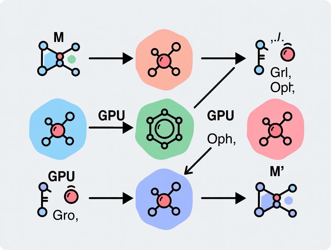
Ecological Network Construction and Optimization Workflow

The following diagram illustrates the integrated workflow for constructing and optimizing an ecological network using GPU-accelerated methods.

GPU Parallel Computing Architecture for Ecological Modeling

This diagram outlines the layered architecture of a GPU-accelerated system for ecological network processing.

Table 3: Key Research Reagents and Resources for Ecological Network Modeling

Item / Resource	Type	Function / Application
InVEST Model	Software Suite	Quantifies and maps multiple ecosystem services (habitat quality, water yield, soil retention) for source identification.
CLUE-S Model	Software	Simulates land-use change scenarios under different developmental policies.
MCR Model	Algorithm	Calculates the least-cost paths for species movement, used to delineate ecological corridors.
Biomimetic Algorithms (PSO, ACO)	Algorithm	Solves high-dimensional nonlinear global optimization problems for land-use layout retrofits.
GPU (NVIDIA L4/Tesla)	Hardware	Provides massive parallel processing capabilities to accelerate computationally intensive spatial optimizations.
NCCL Library	Software Library	Enables high-performance multi-GPU communication for large-scale ecological simulations across compute nodes.
CUDA/OpenACC	Programming Framework	Provides the interface and directives for programming NVIDIA GPUs and parallelizing code.
Fuzzy C-Means Clustering	Algorithm	Identifies potential ecological stepping stones in a global structural optimization process.

Graphics Processing Units (GPUs) have undergone a profound transformation from specialized hardware for rendering images to foundational pillars of general-purpose scientific computation. This evolution is driven by the GPU's inherent massively parallel architecture, which contains hundreds or thousands of processing cores capable of simultaneously executing thousands of threads [6] [7]. This parallel design offers a dramatic performance advantage over traditional Central Processing Units (CPUs) for computational problems that can be structured for parallel execution.

The field of ecological network optimization exemplifies this computational shift. The construction and optimization of Ecological Networks (ENs) is crucial for mitigating habitat fragmentation and achieving coordination between regional development and ecological protection [1] [8]. However, these processes involve computationally intensive tasks, such as simulating ecological processes across large spatial domains and iteratively optimizing complex network structures. The computational efficiency of traditional serial programs often fails to meet the demands of real-time, high-resolution simulation and optimization [7]. Consequently, GPU parallel computing has emerged as a critical enabling technology, allowing researchers to solve ecological network problems that were previously intractable within feasible timeframes [1].

This article details the application of GPU parallel computing to scientific research, with a specific focus on protocols and methodologies for ecological network optimization. We provide quantitative performance comparisons, detailed experimental protocols, and essential toolkits to equip researchers with the practical knowledge needed to leverage GPU acceleration in their computational workflows.

Quantitative Performance Benchmarks

The transition to GPU computing is justified by substantial performance gains across diverse scientific domains. The table below summarizes documented speedup factors achieved by GPU-accelerated applications compared to conventional CPU-based implementations.

Table 1: Performance Benchmarks of GPU-Accelerated Scientific Applications

Application Field	Specific Model/Task	CPU Baseline	GPU Performance	Speedup Factor	Key Enabling Technology
Ocean Modeling [4]	SCHISM Model (Large-scale)	Single CPU node	Single GPU (NVIDIA A100)	35.13x	CUDA Fortran
Network Analysis [9]	Betweenness Centrality	Single-threaded C++	NVIDIA Tesla C2050	10-50x	CUDA C
Concrete Simulation [7]	Temperature Control Simulation	Serial Program	GPU with Async. Parallelism	61.42x	CUDA Fortran
Ecological Network Optimization [1]	Land-use Layout Retrofit	Serial Biomimetic Algorithm	GPU Parallel (MACO Model)	City-level high-resolution optimization enabled	CUDA/CPU Heterogeneous Architecture

These benchmarks demonstrate that GPU acceleration can yield order-of-magnitude improvements in computational efficiency. This performance is critical for ecological research, where high-resolution, dynamic simulations of landscape processes were previously limited by computational bottlenecks. GPU acceleration now enables city-level ecological network optimization at a patch-level resolution, facilitating more nuanced and scientifically robust planning decisions [1].

Experimental Protocols for GPU-Accelerated Ecological Network Optimization

The following section provides a detailed, actionable protocol for implementing a GPU-accelerated ecological network optimization framework, based on the methodology described by Tong et al. [1].

Protocol: Spatial-Operator Based MACO Model for EN Optimization

I. Objective To synergistically optimize the function and structure of Ecological Networks (ENs) at the patch level by coupling spatial operators and a modified ant colony optimization (MACO) algorithm, leveraging GPU parallel computing for high-resolution, city-level simulation.

II. Experimental Workflow and Materials

Table 2: Research Reagent Solutions for GPU-Accelerated EN Optimization

Category	Item/Solution	Function/Description	Example Sources/Tools
Computational Hardware	GPU Accelerator	Provides massive parallel processing cores for fine-grained spatial computations.	NVIDIA Tesla, GeForce RTX series
	High-Performance CPU	Manages serial tasks and coordinates GPU operations.	Multi-core processors (e.g., Intel Xeon)
Software & Programming	CUDA Fortran / CUDA C	Primary programming platforms for developing GPU-accelerated code.	PGI Compiler, NVIDIA Nsight
	Parallel Computing APIs	Enable management of parallel execution across different hardware architectures.	CUDA, OpenCL, OpenACC
Data Inputs	Land Use/Land Cover (LULC) Data	Raster data used to identify ecological sources and calculate resistance surfaces.	National Land Survey Data, Remote Sensing Imagery
	Ecological Sensitivity & Function Metrics	Data layers used to assess habitat quality and identify priority conservation areas.	Soil, Topographic, Meteorological data
Core Algorithms	Morphological Spatial Pattern Analysis (MSPA)	Identifies core ecological patches and structural elements from LULC data.	GuidosToolbox
	Circuit Theory	Models ecological flows and identifies corridors and pinch points.	Circuitscape
	Biomimetic Intelligent Algorithm (MACO)	Optimizes land-use layout for enhanced EN connectivity and function.	Custom implementation [1]

III. Step-by-Step Procedure

• EN Construction and Identification a. Data Preparation: Collect and pre-process multi-source data, including land use/land cover (LULC) maps, remote sensing imagery, and ecological sensitivity indicators. Rasterize all data to a consistent, high resolution (e.g., 40m) [1]. b. Ecological Source Identification: Determine ecological sources through a combined assessment of ecological function (e.g., habitat quality, water conservation) and sensitivity. Use Morphological Spatial Pattern Analysis (MSPA) to identify core landscape patterns from LULC data [8]. c. Resistance Surface Modeling: Construct a comprehensive resistance surface by weighting various natural and anthropogenic factors (e.g., topography, human footprint) [8]. d. Corridor and Node Extraction: Apply circuit theory to extract ecological corridors and identify key strategic nodes (barrier points, pinch points) based on cumulative resistance and current flow patterns [8].

• GPU-Accelerated Optimization Setup a. Algorithm Selection and Modification: Implement a Modified Ant Colony Optimization (MACO) algorithm. The algorithm should incorporate two types of spatial operators: * Micro Functional Optimization Operators: Four operators for bottom-up, patch-level land use adjustment. * Macro Structural Optimization Operator: One operator for top-down identification of potential ecological stepping stones [1]. b. GPU Kernel Development: Port the computationally intensive sections of the MACO algorithm to the GPU using CUDA Fortran or CUDA C. This involves: * Designing the parallel execution configuration (number of thread blocks and threads per block). * Allocating and managing GPU device memory for large geospatial data arrays. * Implementing kernel functions that execute the spatial operators concurrently across thousands of threads [1] [7]. c. Integration of Emergence Mechanism: Develop a global ecological node emergence mechanism using an unsupervised Fuzzy C-Means (FCM) clustering algorithm. This mechanism, running on the GPU, identifies potential areas for ecological stepping stones based on optimization probability, enhancing global connectivity [1].

• Execution and Performance Optimization a. Leverage Heterogeneous Architecture: Establish an efficient data transfer pattern between the CPU (host) and GPU (device) to minimize communication overhead. b. Employ Parallel Computing Techniques: Utilize GPU-based parallel computing techniques to ensure every geographic unit participates in the optimization calculation concurrently and synchronously. For further efficiency, consider using CUDA Streams to overlap data transfer and kernel execution [1] [7]. c. Model Execution: Run the spatial-operator based MACO model on the GPU. The model will dynamically simulate land-use changes and output optimized EN configurations.

• Validation and Analysis a. Evaluation: Assess the optimized EN using predefined evaluation indicators for both functional orientation (e.g., ecosystem service value) and structural orientation (e.g., connectivity indexes, network complexity) [1]. b. Robustness Testing: Test the stability and resilience of the optimized EN against both random and targeted disturbances to evaluate its long-term effectiveness [8].

Diagram 1: Workflow for GPU-accelerated ecological network optimization, highlighting the core computational phase performed on the GPU.

Advanced Technical Implementation and Optimization

Achieving peak performance in GPU-accelerated applications requires careful attention to memory management, parallel execution patterns, and communication protocols.

Memory Hierarchy and Access Optimization

GPU memory architecture includes global, shared, and register memory. Efficient use of shared memory is critical for performance, as it offers much higher bandwidth and lower latency than global memory.

• Protocol: Matrix Transposition using Shared Memory [7]
  • Objective: Accelerate a matrix transposition subroutine, a common operation in solvers.
  • Procedure: a. Each thread block is assigned a tile (e.g., 32x32 elements) of the source matrix. b. All threads within the block collaboratively load the assigned tile from global memory into shared memory. c. Threads synchronize to ensure the entire tile is loaded. d. Threads write the data from shared memory to the destination matrix in the transposed layout.
  • Optimization: Address bank conflicts in shared memory by padding the shared memory array or using appropriate access patterns. This optimization alone has been shown to achieve speedups of 437.5x for matrix transposition [7].

Asynchronous Execution and Concurrent Data Transfer

To further hide the latency of data transfers between the CPU and GPU, asynchronous execution patterns can be employed.

• Protocol: Asynchronous Parallelism with CUDA Streams [7]
  • Objective: Overlap data transfer time with kernel execution time to improve overall computational efficiency.
  • Procedure: a. Create multiple CUDA streams. b. Divide the input data into chunks. c. For each chunk: * Use cudaMemcpyAsync in a specific stream to copy the chunk from host to device. * Launch a processing kernel in the same stream to operate on the chunk already in device memory. * Use cudaMemcpyAsync to copy the result back to the host. d. This pipeline allows data transfer for chunk n+1 to occur concurrently with kernel execution for chunk n.
  • Result: This method can double the computing efficiency compared to a basic GPU-parallel implementation, leading to a 61.42x speedup over the original serial program for inner product matrix multiplication [7].

Multi-GPU and Large-Scale Cluster Communication

For problems exceeding the memory or computational capacity of a single GPU, scaling across multiple GPUs or nodes is necessary. The NVIDIA Collective Communication Library (NCCL) is essential for this task.

• Protocol: Multi-GPU Collective Communication with NCCL [5]
  • Objective: Perform efficient collective operations (e.g., All-Reduce) across multiple GPUs in a cluster.
  • Procedure: a. Communicator Management: Initialize an NCCL communicator that defines the set of GPUs participating in the communication using ncclCommInitAll (single process) or ncclCommInitRank (multi-process). b. Algorithm Selection: NCCL internally selects efficient algorithms (e.g., ring or tree-based) and protocols (Simple, LL, LL128) based on message size and system topology to optimize bandwidth and latency [5]. c. Operation Launching: Call the collective operation (e.g., ncclAllReduce) within the established communicator. Use ncclGroupStart and ncclGroupEnd to aggregate operations and reduce launch overhead. d. Cleanup: Safely destroy the communicator with ncclCommDestroy after operations complete.

Diagram 2: GPU execution and memory model, illustrating the relationship between host code, kernel execution, and the critical memory hierarchy on the device.

The journey of GPU parallel computing from a graphics-specific tool to a cornerstone of general-purpose scientific computation has fundamentally expanded the scope of problems researchers can tackle. In the specific context of ecological network optimization, GPU acceleration enables high-resolution, dynamic, and quantitatively rigorous simulations that directly inform conservation planning and ecosystem management. The protocols and performance data outlined herein provide a roadmap for researchers to harness this computational power. As GPU hardware and programming models like CUDA continue to evolve, their role in solving complex scientific and environmental challenges will only become more pronounced.

Why GPUs? Understanding Massively Parallel Architecture for Ecological Optimization Problems

Quantitative Analysis of GPU Performance and Impact

The adoption of GPU computing for ecological optimization is driven by quantifiable performance gains and specific architectural advantages. The tables below summarize key performance metrics and environmental considerations.

Table 1: GPU Performance Acceleration in Scientific Modeling

Application Domain	Specific Model/Task	CPU Baseline	GPU-Accelerated Performance	Achieved Speedup	Key Factor for Speedup
Geological Anisotropy Analysis [10]	Every-direction Variogram Analysis (EVA)	Serial CPU Implementation	GPU Implementation	~42x	Embarrassingly parallel grid computation
Bird Migration Simulation [10]	Agent-Based Model (Bird Flight)	Serial CPU Implementation	GPU Implementation	~1.5x	Parallel processing of independent agents
Topology Optimization [11]	3D Linear Elastic Compliance Minimization	48 CPU Cores (~3.17 hours)	Single GPU (~2 hours)	~1.6x (faster)	Parallel processing of ~65.5 million elements
General Climate Modeling [12]	AI/ML Inference Benchmarks	Advanced CPU	NVIDIA A100 GPU	237x	Massive parallelization of AI workloads

Table 2: GPU Operational Characteristics and Environmental Impact

Metric	Value / Range	Context & Explanation
Thermal Design Power (TDP) [13]	15 - 2,400 Watts	Range for workstation GPUs (post-2020); outliers like Intel's Data Center GPU Max Subsystem reach 2,400W.
Idle Power Consumption [13]	~20% of TDP	AI servers idle at roughly 20% of their rated power, highlighting base energy draw.
Embodied Carbon per GPU Card [13]	141 - 585 kg CO₂e	Carbon dioxide equivalent emissions from manufacturing; varies by study and card model. NVIDIA H100: ~164 kg CO₂e [13].
Projected Global Electricity Consumption [14]	Up to 8% by 2030	Projected share for AI and high-performance computing (HPC), underscoring the scale of GPU-driven energy demand.

Experimental Protocols for GPU-Accelerated Ecological Optimization

This section provides a detailed, actionable protocol for implementing a GPU-accelerated ecological network optimization, synthesing methodologies from recent research.

Protocol 1: Coupling Spatial Operators and Biomimetic Algorithms for EN Optimization

This protocol is adapted from a study optimizing the ecological network (EN) of Yichun City, which integrated microscopic functional optimization with macroscopic structural optimization [1].

2.1 Research Objectives and Preparation

• Objective: To quantitatively and dynamically optimize an ecological network's function and structure at the patch level, answering "Where to optimize, how to change, and how much to change?"
• Preparatory Steps:
  • Define Study Area: The methodology is designed for city-level or urban agglomeration-scale areas [1].
  • Data Collection: Gather high-resolution geospatial data. The foundational study used a 40m resolution land use map derived from the National Land Survey, alongside data on topography, climate, soil, and socio-economic factors [1].
  • Initial EN Construction: Construct a baseline ecological network using standard methods:
    • Ecological Sources: Identify via ecological function and sensitivity assessment, followed by Morphological Spatial Pattern Analysis (MSPA) [1].
    • Corridors and Nodes: Extract using ecological connectivity analysis and circuit theory [1].

2.2 Computational Hardware and Software Setup

• Hardware: A computing system with a modern GPU. The protocol leverages GPU/CPU heterogeneous architecture [1].
• Software & Frameworks:
  • Programming Language: C, C++, or Python are suitable due to their support for GPU programming and large scientific communities [10].
  • Parallel Computing API: OpenCL (for vendor-agnostic code) or NVIDIA's CUDA (for optimal performance on NVIDIA hardware) [1] [15].
  • Algorithm Implementation: Implement the modified Ant Colony Optimization (ACO) algorithm or other biomimetic algorithms (e.g., Particle Swarm Optimization) as the core optimization engine [1].

2.3 Implementation of the Optimization Model The core of the protocol is a spatial-operator-based Multi-objective ACO (MACO) model.

• Define Objective Functions: Formulate two primary objectives for the algorithm to pursue simultaneously:
  • Functional Optimization: Maximize the overall ecological function of the landscape (e.g., habitat quality, ecosystem services) [1].
  • Structural Optimization: Maximize the structural connectivity of the EN (e.g., by improving connectivity between ecological patches) [1].
• Incorporate Land-Use Constraints: Define constraints within the model, such as total available land for conversion and land-use suitability, to ensure results are practical [1].
• Apply Spatial Optimization Operators: The MACO model uses several operators to guide the optimization:
  • Four Micro Functional Operators: Bottom-up operators that handle fine-scale, patch-level land-use adjustments for functional enhancement [1].
  • One Macro Structural Operator: A top-down operator that identifies and prioritizes the creation of new "ecological stepping stones" in strategically important global locations to improve overall network connectivity [1].
• Enable GPU Parallelization: Implement the model to run on the GPU. The key is to ensure that calculations for each geographic unit (e.g., grid cell) are processed concurrently and synchronously by the GPU's thousands of cores [1] [10]. This involves establishing an efficient data transfer pattern between the CPU and GPU.

2.4 Validation and Analysis

• Performance Evaluation: Compare the optimized EN against the baseline using pre-defined quantitative metrics for both function and structure [1].
• Computational Benchmarking: Record the time taken for the GPU-accelerated optimization and compare it against a serial CPU implementation if possible, to quantify the speedup [10].
• Spatial Output Analysis: Interpret the final optimized map, which provides a patch-level land-use adjustment plan, specifying the location, type, and extent of changes needed [1].

Protocol 2: GPU-Acceleration of Spatially-Explicit Ecological Models

This protocol provides a generalized framework for porting classic ecological models to GPUs, based on established practices in the field [15].

2.1 Problem Definition and Code Selection

• Objective: To significantly accelerate the simulation of a spatially-explicit ecological model (e.g., patterns in mussel beds, arid vegetation).
• Preparatory Steps:
  • Select a Model: Choose a model where the state of each cell in a grid depends only on its neighbors, making it suitable for parallelization.
  • Obtain Code: Start with an existing, validated serial code (e.g., in C, C++) for which the dynamics are well-understood [15].

2.2 Implementation for GPU Execution

• Grid Representation: Represent the spatial landscape as a 2D or 3D grid in the GPU's memory (VRAM). The high memory bandwidth of GPUs is critical for efficiently handling this data [12].
• Kernel Function Development: The core computational logic (e.g., calculating growth, mortality, interaction between species) is written as a "kernel." This kernel is a function that is executed simultaneously by thousands of GPU threads.
• Thread Per Cell Mapping: Design the kernel so that a single GPU thread is responsible for performing the model calculations for a single cell (or a small block of cells) in the spatial grid. This maps the natural parallelism of the problem to the GPU architecture [15].
• Neighborhood Handling: Program the kernel to efficiently access the state of neighboring cells, which is essential for modeling spatial feedback and diffusion processes.

2.3 Execution and Simulation

• Data Transfer: Copy the initial state of the model grid from the CPU's main memory to the GPU's VRAM.
• Kernel Launch: For each time step of the simulation, launch the kernel on the GPU. The GPU automatically executes the kernel across all threads in parallel.
• Result Retrieval: After the simulation is complete, or at intervals for saving snapshots, copy the final state of the grid from the GPU back to the CPU.

Visualizing Workflows and System Architecture

The following diagrams, generated using Graphviz, illustrate the logical relationships and workflows described in the protocols.

Diagram 1: High-Level Research Workflow

Diagram 2: GPU vs. CPU Architectural Paradigm

The Scientist's Toolkit: Essential Research Reagents and Solutions

This table details the key hardware, software, and data "reagents" required for conducting GPU-accelerated ecological optimization research.

Table 3: Essential Research Reagents for GPU-Accelerated Ecological Optimization

Category	Item / Solution	Function / Purpose in Research
Hardware	High-Performance GPU (e.g., NVIDIA A100, H100)	Provides the core parallel processing power for accelerating complex simulations and optimization algorithms [12] [16].
Hardware	Adequate System Memory (RAM) & VRAM	Ensures the system can hold and rapidly process large, high-resolution geospatial datasets and model states [12].
Software & APIs	Parallel Computing API (CUDA, OpenCL)	Provides the programming interface to write code that executes on the GPU hardware [15] [10].
Software & APIs	Scientific Computing Libraries (e.g., CuPy, RAPIDS)	Offers GPU-accelerated versions of common mathematical and data science operations, speeding up development [17].
Software & APIs	Machine Learning Frameworks (e.g., TensorFlow, PyTorch with GPU support)	Used for developing and training AI-powered climate emulators or surrogate models within the optimization workflow [12] [17].
Data & Models	High-Resolution Geospatial Data	Serves as the foundational input for constructing and validating ecological networks and spatial models [1].
Data & Models	Validated Serial Model Code	Provides a correct, baseline implementation of the ecological model to be parallelized and used for verifying GPU-accelerated results [15].

The concurrent crises of biodiversity loss and protracted biomedical discovery timelines represent critical challenges for global sustainability and human health. While these fields appear distinct, they are increasingly united by a common dependency on advanced computational solutions. High-performance computing (HPC), particularly GPU-accelerated parallel processing, is emerging as a transformative tool for addressing the data-intensive modeling and simulation requirements in both ecology and biomedicine. In ecology, habitat fragmentation driven by human activities damages ecological connectivity and undermines ecosystem resilience [1]. In biomedicine, the complexity of biological systems demands computational power that can scale with the volume of omics and clinical data. This application note details how GPU technologies enable high-fidelity simulations of ecological networks and accelerate therapeutic discovery, providing detailed protocols for researchers in both domains.

Habitat Fragmentation: Ecological Crisis and Computational Solutions

The Problem and Its Impacts

Habitat fragmentation, characterized by the disassembly of continuous habitats into smaller, isolated patches, is a primary driver of global biodiversity decline. It involves two distinct components: habitat loss (overall reduction in habitat area) and fragmentation per se (the breaking apart of habitat independent of total area loss) [18]. The ecological consequences are severe:

• Impaired Ecosystem Function: Habitat loss weakens the positive relationship between plant richness and above-ground biomass in grasslands, directly reducing carbon storage and ecosystem productivity [18].
• Increased Extinction Risk: For terrestrial mammals, the degree of habitat fragmentation is a stronger predictor of extinction risk transition than life-history traits or general human pressure variables [19].
• Matrix Condition Mediation: The condition of the surrounding landscape matrix critically determines fragmentation impacts. High human pressure in the matrix (e.g., intensive agriculture, urbanization) exacerbates extinction risks, while lower-pressure matrices can mitigate them [19].
• Disease Emergence Risk: Fragmented landscapes with complex boundaries increase human exposure to wildlife microbes, potentially elevating the risk of novel infectious disease emergence [20].

Table 1: Ecological Impacts of Habitat Fragmentation Components

Fragmentation Component	Primary Ecological Effect	Impact on Biodiversity
Habitat Loss	Decreases plant richness [18]	Reduces specialist species [18]
Fragmentation Per Se	Increases plant richness but decreases above-ground biomass [18]	Alters species composition
Matrix Degradation	Increases patch isolation effects [19]	Heightens extinction risk for specialists [19]
Edge Effects	Alters microclimate and species interactions	Promotes generalist species

GPU-Accelerated Ecological Network Optimization

Traditional ecological network optimization approaches have struggled to simultaneously address functional and structural constraints. A groundbreaking methodology couples spatial operators with biomimetic intelligent algorithms (e.g., Modified Ant Colony Optimization, MACO) within a GPU-accelerated framework [1]. This approach synergizes bottom-up functional optimization with top-down structural optimization through:

• Micro-functional Optimization Operators: Four patch-level operators that adjust local land use patterns to enhance ecological function.
• Macro-structural Optimization Operator: A single landscape-level operator that identifies potential ecological stepping stones using unsupervised fuzzy C-means clustering to improve overall connectivity [1].
• GPU-CPU Heterogeneous Architecture: Parallel computing techniques that enable city-level ecological optimization at high spatial resolution by ensuring "every geographic unit can participate in the optimization calculation concurrently and synchronously" [1].

This computational framework dynamically answers critical planning questions: "Where to optimize, how to change, and how much to change?" providing quantitative guidance for conservation prioritization [1].

Biomedical Discovery: The High-Performance Computing Imperative

Computational Challenges in Biomedicine

Biomedical research faces exponentially growing computational demands across multiple domains:

• Multi-scale Biological Modeling: Integrating molecular, cellular, and organ-level simulations requires enormous computational resources [21].
• Large-Scale Omics Data Analysis: Genome sequencing and proteomic datasets present substantial processing bottlenecks [22].
• Precision Medicine Applications: Developing patient-specific "digital twins" necessitates rapid, high-fidelity simulations of physiological processes [21].

GPU-Accelerated Biomedical Breakthroughs

The Center for Precision Medicine and Data Sciences (CPMDS) at UC Davis exemplifies GPU-enabled biomedical innovation, using HPC resources to:

• Simulate large protein systems, including voltage-gated ion channels, to study modulator influences on structure and function [21].
• Analyze large-scale omics datasets to identify disease-related genes, proteins, and networks.
• Develop predictive AI models capturing genetic variant effects and simulate populations of synthetic cardiomyocytes to model electrophysiological variability and drug sensitivity [21].

As CPMDS researchers note, "Deep learning frameworks depend on GPU acceleration to train models on terabytes of synthetic cell simulations," enabling clinically relevant predictive modeling that would be "impractical without HPC" [21].

Experimental Protocols and Workflows

Protocol: GPU-Accelerated Ecological Network Optimization

Application: Optimizing ecological network function and structure in fragmented landscapes.

Required Resources: Land use/land cover data, species distribution data, remote sensing imagery, high-performance computing environment with GPU capabilities.

Methodology:

• Ecological Source Identification:

  • Conduct ecological function and sensitivity assessments using spatial analytics.
  • Apply Morphological Spatial Pattern Analysis (MSPA) to identify core habitat patches.
  • Calculate ecological connectivity indices using graph theory metrics.

• Spatial-Operator Based MACO Model Setup:

  • Implement four micro-functional optimization operators for patch-level land use adjustment.
  • Configure one macro-structural optimization operator with fuzzy C-means clustering for stepping stone identification.
  • Define objective functions balancing ecological connectivity and land use suitability.

• GPU Parallelization:

  • Establish data transfer patterns between CPU and GPU using CUDA or OpenACC frameworks.
  • Implement parallel processing of geographic units using thousands of concurrent threads.
  • Optimize memory bandwidth usage for large geospatial datasets.

• Optimization Execution:

  • Run biomimetic algorithm iterations with simultaneous functional and structural optimization.
  • Validate results against conservation targets and spatial constraints.
  • Generate spatial explicit land use adjustment recommendations with quantitative change amounts.

Computational Note: The GPU-CPU heterogeneous architecture enables city-level optimization at 40m resolution, processing over 24 million grids concurrently [1].

Diagram 1: Ecological Network Optimization Workflow

Protocol: GPU-Accelerated Biomedical Simulation

Application: Precision medicine and drug discovery through multi-scale biological modeling.

Required Resources: Omics datasets, protein structures, clinical data, HPC environment with NVIDIA GPUs, molecular dynamics software (e.g., GROMACS, NAMD), deep learning frameworks (e.g., TensorFlow, PyTorch).

Methodology:

• System Preparation:

  • For molecular simulations: obtain protein structures from Protein Data Bank, prepare topology files, solvate systems, and apply boundary conditions.
  • For omics analysis: preprocess raw sequencing data, perform quality control, and generate normalized expression matrices.
  • For digital twin development: integrate physiological parameters, medical imaging data, and clinical biomarkers.

• GPU-Accelerated Computation:

  • Molecular Dynamics: Offload force calculations and particle mesh Ewald electrostatics to GPU using CUDA-accelerated codes.
  • Deep Learning: Utilize GPU tensor cores for training neural networks on terabyte-scale simulation datasets.
  • Implement CUDA kernels for customized biological algorithms and analysis pipelines.

• Multi-Scale Integration:

  • Couple molecular simulation outputs with cellular-scale models through parameterization.
  • Integrate cellular models into tissue and organ-level simulations.
  • Validate multi-scale predictions against experimental and clinical observations.

• Analysis and Prediction:

  • Apply AI surrogate models to rapidly predict system behavior across parameter spaces.
  • Identify critical disease mechanisms and therapeutic targets.
  • Generate patient-specific treatment predictions and risk assessments.

Implementation Tip: Researchers new to HPC should "start with small test jobs before scaling to larger workflows, learn the basics of SLURM early, document pipelines carefully, and take advantage of available HPC training and support" [21].

Diagram 2: Biomedical Discovery Computational Pipeline

Performance Metrics and Accelerated Outcomes

Computational Performance Gains

GPU acceleration delivers transformative performance improvements across both ecological and biomedical domains:

Table 2: Computational Performance Improvements with GPU Acceleration

Application Domain	Traditional CPU Performance	GPU-Accelerated Performance	Speedup Factor
Ecological Network Optimization	Serial processing of geographic units [1]	Concurrent synchronous processing of all units [1]	City-level optimization now feasible
SCHISM Ocean Model	CPU-based finite element computation [4]	GPU-accelerated Jacobi solver [4]	35.13x (2.56M grid points)
Cardiac Electrophysiology	Workstation-scale simulation [21]	HPC-enabled digital twin modeling [21]	Months to days conversion
Computational Fluid Dynamics	CPU-based CFD simulation [23]	GPU-accelerated CFD with AI surrogates [23]	10x faster
Bioinformatics Variant Calling	CPU-based processing [22]	NVIDIA Parabricks GPU acceleration [22]	>60% cost savings

Scientific and Conservation Outcomes

Beyond computational metrics, GPU acceleration enables substantive scientific advances:

• Ecological: Identification of optimal locations for ecological stepping stones and quantitative guidance for patch-level land use adjustments, enhancing landscape connectivity [1].
• Biomedical: Prediction of arrhythmia risk from electrophysiology data, revelation of novel drug mechanisms through protein-modulator interaction simulations, and population-scale analysis of genetic variant effects [21].
• Cross-disciplinary: AI surrogate models achieving 3,600x speedup for methane leak detection (energy sector) and 10x acceleration in porosity field prediction (geology) demonstrate the transferability of these approaches [23].

Table 3: Key Research Reagent Solutions for Computational Ecology and Biomedicine

Resource Category	Specific Tools & Platforms	Primary Function	Application Domain
Hardware Platforms	NVIDIA Blackwell GPUs [23]	Massively parallel computation	Both
Software Libraries	CUDA-X, OpenACC [23] [24]	GPU programming frameworks	Both
Ecological Modeling	Spatial-operator based MACO [1]	Ecological network optimization	Ecology
Biomedical Analysis	NVIDIA Parabricks [22]	Genomic variant calling	Biomedicine
Molecular Simulation	GROMACS, NAMD	Molecular dynamics	Biomedicine
Collaboration Platforms	NVIDIA Omniverse [23]	Real-time 3D collaboration	Both
Workflow Management	Nextflow [22]	Pipeline orchestration	Both
HPC Orchestration	SLURM [21]	Job scheduling and resource management	Both

GPU parallel computing has evolved from a specialized technology to an essential enabling platform addressing critical challenges in both ecology and biomedicine. The methodologies detailed herein provide actionable pathways for researchers to implement these advanced computational approaches, transforming previously intractable problems into solvable challenges. As GPU technologies continue to advance with architectures like NVIDIA Blackwell offering 150x more compute power, the potential for cross-disciplinary innovation expands considerably [23]. By adopting these GPU-accelerated frameworks, researchers can dramatically accelerate the pace of discovery while addressing urgent sustainability and health challenges through high-fidelity simulation and predictive modeling.

Core Conceptual Framework and Quantitative Definitions

Ecological networks (ENs) are foundational to mitigating habitat degradation and fragmentation caused by rapid urbanization. They function as interconnected systems that enhance ecosystem resilience and maintain regional ecological processes by facilitating species movement [1]. The table below defines the core components and their quantitative descriptors.

Table 1: Core Components of an Ecological Network

Component	Definition	Key Quantitative Metrics
Ecological Patches	Habitats that serve as sources for species dispersal and provide ecosystem services [25].	Area, shape index, habitat quality index, importance value (dPC).
Ecological Corridors	Spatial pathways that connect ecological patches, facilitating the flow of species, energy, and material [25].	Width, length, cost-weighted distance, current flow (from circuit theory).
Ecological Connectivity	The functional measure of how landscape structure facilitates or impedes movement between resource patches [1].	Probability of Connectivity (PC), Integral Index of Connectivity (IIC), Equivalent Connectivity (EC).
Computational Stencils	In high-performance computing, data transfer patterns between CPU and GPU that enable geographic units to participate in optimization concurrently [1].	Spatial resolution (e.g., 40m grid cells), number of parallel processing threads, memory bandwidth.

Computational Analysis and Optimization Protocols

Protocol: Constructing a Landscape Ecological Network (LEN)

This protocol outlines the methodology for identifying and connecting ecological patches to form a foundational ecological network [25].

1. Identify Ecological Sources:

• Data Inputs: Land Use/Land Cover (LULC) map, Normalized Difference Vegetation Index (NDVI), Digital Elevation Model (DEM).
• Procedure: a. Conduct a habitat suitability assessment, integrating factors like vegetation cover, human disturbance, and topography. b. Apply Morphological Spatial Pattern Analysis (MSPA) to the suitability map to identify core habitat areas. c. Evaluate the connectivity importance of each core patch using a probability of connectivity (PC) index in software such as Conefor. d. Select patches with the highest importance values as final ecological sources.

2. Develop an Ecological Resistance Surface:

• Data Inputs: LULC map, road network, population density, topographic data.
• Procedure: a. Assign a resistance value (e.g., 1-100) to each landscape feature based on its perceived impedance to species movement (e.g., high for urban land, low for forests). b. Create a composite resistance surface using a GIS, integrating all weighted factors.

3. Delineate Ecological Corridors:

• Tools: Linkage Mapper, Circuitscape, or least-cost path algorithms in GIS.
• Procedure: a. Use a Minimum Cumulative Resistance (MCR) model to calculate the least-cost path between pairs of ecological sources. b. Alternatively, apply circuit theory to identify pinch points and movement pathways across the entire landscape.

Protocol: Optimizing an Ecological Network using a Biomimetic Intelligent Algorithm

This protocol details a advanced method for the synergistic, patch-level optimization of an EN's function and structure using a modified ant colony optimization (MACO) algorithm [1].

1. Define the Optimization Framework:

• Objective Functions:
  • Function-oriented: Maximize total habitat quality/function of all ecological patches.
  • Structure-oriented: Maximize the global connectivity (e.g., IIC) of the entire network.
• Constraint Conditions: Set constraints for total area of ecological land, maximum budget for land-use conversion, and spatial adjacency rules.
• Transformation Rules: Define land-use transition rules (e.g., how farmland can be converted to ecological land).

2. Implement Spatial Optimization Operators:

• Integrate the following operators into the MACO algorithm: a. Micro Functional Optimization Operators (Bottom-up): Adjust local land-use patterns to improve the ecological function of individual patches. b. Macro Structural Optimization Operator (Top-down): Identifies potential new ecological stepping stones globally to enhance overall network connectivity. c. Global Ecological Node Emergence: Uses the Fuzzy C-Means (FCM) clustering algorithm to identify locations with high potential to become new ecological sources.

3. Execute GPU-Accelerated Parallel Computation:

• Hardware: Utilize consumer-grade high-performance Graphics Processing Units (GPUs).
• Software: Implement using parallel computing frameworks like CUDA or OpenCL.
• Procedure: a. Establish a data transfer pattern (computational stencil) between the CPU and GPU. b. Distribute the optimization calculation for every geographic unit (e.g., grid cell) across thousands of parallel GPU threads. c. Run the MACO model synchronously and concurrently on all units to identify the optimal land-use retrofit plan.

Table 2: Key Metrics for Evaluating Network Optimization Performance

Evaluation Orientation	Performance Metric	Description
Functional Optimization	Habitat Quality Index	Measures the capacity of a patch to support species, based on its intrinsic characteristics and surrounding threats.
Structural Optimization	Integral Index of Connectivity (IIC)	A graph-based metric that evaluates the overall connectivity of the network based on the topology of patches and links.
Computational Efficiency	Speed-up Ratio	The ratio of computation time on a CPU to the computation time on a GPU for the same optimization task.

Visual Workflows and System Architecture

Ecological Network Construction & Optimization

GPU-Accelerated Optimization Stencil

Table 3: Essential Tools and Platforms for Ecological Network Research

Tool/Resource	Category	Primary Function	Reference
Conefor	Stand-alone / R-based	Quantifies the importance of habitat patches for landscape connectivity using graph theory.	[25] [26]
Linkage Mapper	ArcGIS Toolbox	A GIS toolset to model ecological corridors using least-cost path analysis.	[26]
Circuitscape	Stand-alone / GIS	Applies circuit theory to model landscape connectivity and identify movement corridors.	[25] [26]
GECOT	Open-source Tool	Models conservation and restoration planning as a connectivity optimization problem under budget constraints.	[26]
CUDA/OpenCL	Parallel Computing Framework	APIs for enabling parallel computing on NVIDIA (CUDA) or cross-vendor (OpenCL) GPUs.	[1] [6]
Fuzzy C-Means (FCM)	Algorithm	Unsupervised clustering used to identify potential new ecological nodes in optimization models.	[1]
Ant Colony Optimization (ACO)	Biomimetic Algorithm	A metaheuristic optimization algorithm inspired by ant foraging behavior, used for land-use layout retrofits.	[1]

Building and Deploying GPU-Optimized Ecological Models

Ecological network optimization research has entered a data-intensive era, where understanding complex spatiotemporal patterns requires immense computational power. Modern studies, such as those analyzing the spatiotemporal evolution of ecological networks in arid regions, involve processing decades of satellite imagery, climate data, and species distribution information. These analyses generate massive datasets with trillions of grid points and quadrillion-degree-of-freedom simulations that surpass the capabilities of traditional central processing unit (CPU)-based computing. The emergence of graphics processing unit (GPU) parallel computing frameworks has revolutionized this field by enabling researchers to execute complex ecological simulations orders of magnitude faster than previously possible.

GPU computing frameworks provide the essential toolkit for accelerating every stage of ecological modeling, from data preprocessing to simulation and optimization. The parallel architecture of GPUs, featuring thousands of computational cores, is uniquely suited to the embarrasingly parallel nature of many ecological algorithms, including spatial pattern analysis, landscape connectivity modeling, and circuit theory applications. This article provides detailed application notes and experimental protocols for leveraging three key GPU computing frameworks—CUDA, OpenACC, and PyTorch—within the context of ecological network optimization research. By integrating these tools, researchers can achieve unprecedented scale and precision in modeling complex ecological systems, ultimately supporting more effective conservation strategies and ecosystem management decisions.

The GPU Computing Toolkit for Ecological Research

Ecological researchers have multiple pathways for leveraging GPU acceleration, each with distinct advantages for different aspects of ecological modeling. The three primary frameworks discussed herein—CUDA, OpenACC, and PyTorch—represent complementary approaches that can be integrated into a comprehensive research workflow. CUDA provides low-level hardware control for optimizing performance-critical routines, OpenACC offers directive-based acceleration with minimal code modification, and PyTorch enables rapid prototyping of machine learning components for ecological prediction tasks. A comparative analysis of these frameworks reveals their respective positioning within the research toolkit.

Table 1: Comparison of GPU Computing Frameworks for Ecological Research

Framework	Programming Approach	Primary Use Cases in Ecology	Learning Curve	Performance Optimization
NVIDIA CUDA	C++, Python, Fortran with GPU-specific extensions	High-performance computing for spatial analysis, circuit theory, fluid dynamics simulations	Steep	Maximum performance via direct hardware control
OpenACC	Directives added to C++, Fortran	Accelerating existing ecological simulation code with minimal rewriting	Moderate	Good performance with minimal code modification
PyTorch	Python with GPU tensor operations	Machine learning for species distribution modeling, habitat suitability prediction	Gentle	High performance for ML models, automatic differentiation

The selection of an appropriate framework depends on multiple factors, including the researcher's computational background, existing codebase, and specific modeling requirements. CUDA delivers maximum performance but requires significant programming expertise and code restructuring. OpenACC provides a balanced approach for accelerating existing Fortran, C, or C++ ecological simulations with minimal code changes, making it ideal for legacy codebases. PyTorch offers the most accessible entry point for researchers already familiar with Python and is particularly valuable for integrating machine learning approaches with traditional ecological modeling.

Research Reagent Solutions: Essential Software Components

Implementing GPU-accelerated ecological modeling requires a suite of specialized software components that function as the "research reagents" of computational ecology. These foundational elements provide the mathematical operations, data structures, and programming interfaces necessary to efficiently execute ecological algorithms on GPU hardware. The core components listed below represent the essential toolkit for researchers embarking on GPU-accelerated ecological network optimization.

Table 2: Essential Software Components for GPU-Accelerated Ecological Research

Component	Function	Ecological Application Example
CUDA Toolkit	Development environment for GPU-accelerated applications	Provides compiler, libraries and runtime for custom ecological algorithms
cuDF	GPU-accelerated DataFrame operations	Accelerating spatial data processing for habitat fragmentation analysis
OpenACC Compiler	Directive translation for automatic GPU parallelization	Accelerating legacy Fortran code for hydrological simulations
PyTorch with CUDA	GPU-accelerated tensor operations and neural networks	Species distribution modeling using deep learning
CUDA-Q	Hybrid quantum-classical computing platform	Future applications in modeling complex ecological networks
Thrust Library	CUDA C++ template library for parallel algorithms	Spatial sorting and searching operations in landscape genetics

These software components interface with specialized hardware to form a complete research environment. The hardware foundation typically includes NVIDIA GPUs (from consumer-grade RTX cards to data center accelerators like the H100), AMD Instinct series GPUs for ROCm-based workflows, or cloud-based GPU instances. For ecological research teams with limited computational expertise, containerization platforms like Docker with the NVIDIA Container Toolkit provide pre-configured environments that eliminate complex dependency management, while services like Thunder Compute offer affordable testing for both CUDA and ROCm frameworks at approximately $0.66-$0.78 per hour for A100 GPUs.

Application Notes: Framework Integration in Ecological Workflows

CUDA for High-Performance Ecological Simulation

The CUDA platform provides the foundational layer for GPU-accelerated ecological modeling, delivering maximum performance for computationally intensive simulations. Ecological research applications that benefit most from CUDA implementation include high-resolution spatial pattern analysis, landscape connectivity modeling, and individual-based simulations with numerous autonomous agents. A recent study on ecological network optimization in Xinjiang from 1990-2020 exemplifies this approach, implementing Morphological Spatial Pattern Analysis (MSPA) and circuit theory with GPU acceleration to process 30 years of satellite-derived vegetation and drought indices [27]. This research, which analyzed changes over 26,438 km² of ecological resistance and 743 km of ecological corridors, required the massive parallelism that CUDA provides.

The CUDA ecosystem offers specialized libraries that directly benefit ecological modeling workflows. The cuDF library, for instance, provides GPU-accelerated DataFrame operations that can dramatically accelerate the preprocessing of ecological tabular data, with performance gains of 10-100× over CPU-based pandas operations for large datasets [28]. For matrix operations fundamental to spatial analysis, the cuBLAS library delivers optimized linear algebra routines, while the Thrust library offers parallel algorithms for sorting, reduction, and prefix-sums that accelerate landscape connectivity analyses. These components enable researchers to construct complete ecological modeling pipelines that remain entirely on the GPU, minimizing costly data transfers between system and GPU memory.

A representative example of CUDA acceleration in ecological modeling can be found in the implementation of circuit theory algorithms for modeling landscape connectivity. Circuit theory, which treats landscapes as electrical circuits where current flow represents movement probability, requires solving systems of linear equations for millions of grid cells. A CUDA implementation parallelizes this process across thousands of GPU cores, reducing computation time from days to hours and enabling higher-resolution analyses. Similarly, individual-based models that simulate the movement of thousands of organisms through heterogeneous landscapes achieve nearly linear scaling with CUDA implementation, allowing researchers to incorporate greater ecological complexity and run more simulations for robust statistical analysis.

OpenACC for Directive-Based Acceleration of Legacy Code

OpenACC provides a directive-based approach to GPU acceleration that is particularly valuable for ecological research groups with substantial investments in legacy Fortran, C, or C++ codebases. Unlike CUDA, which requires rewriting algorithms specifically for GPU execution, OpenACC allows researchers to incrementally accelerate existing code by adding simple compiler directives that identify parallel regions. This approach was demonstrated in the MHIT36 project, where OpenACC directives were used to create a GPU-tailored solver for interface-resolved simulations of multiphase turbulence, achieving excellent scaling efficiency across 1024 GPUs [29]. The directive-based model enables ecological researchers to accelerate complex simulations with minimal code restructuring, preserving decades of validated algorithmic development.

The OpenACC programming model uses #pragma acc directives to specify parallel regions, data movement between host and device memory, and loop-level parallelism. A typical ecological simulation accelerated with OpenACC might include directives to parallelize nested loops that update spatial grid cells, reduce error metrics across the computational domain, and manage the transfer of landscape resistance matrices between CPU and GPU memory. During an Open Hackathon organized by CINECA, this approach delivered a 26× speedup for the MHIT36 solver [29], demonstrating the significant performance gains possible with directive-based acceleration. Similar benefits have been realized in ecological applications, where OpenACC has been used to accelerate wind farm wake modeling in the FLORIS simulator, achieving 190× speedup for a real-world challenge problem [29].

The OpenACC ecosystem supports researchers through specialized training events, hackathons, and bootcamps designed to build proficiency with directive-based programming. These resources are particularly valuable for ecological research teams that may have extensive domain expertise but limited parallel programming experience. The OpenACC specification continues to evolve, with ongoing development focused on improving performance portability across diverse accelerator architectures, including AMD and Intel GPUs. This architectural diversity is increasingly important for ecological researchers seeking to maximize computational efficiency on different supercomputing platforms, such as Frontier (AMD GPUs), Aurora (Intel GPUs), and Polaris (NVIDIA GPUs) [29].

PyTorch for Machine Learning in Ecological Prediction

PyTorch has emerged as the leading framework for integrating machine learning approaches with ecological modeling, particularly for tasks involving pattern recognition, species distribution prediction, and habitat suitability assessment. The framework's intuitive interface, automatic differentiation capabilities, and extensive ecosystem of pre-trained models enable ecological researchers to rapidly develop and deploy deep learning solutions without low-level GPU programming. PyTorch's support for both CUDA and ROCm backends ensures broad hardware compatibility, from individual workstations with consumer GPUs to large-scale computing clusters with enterprise accelerators [30].

Ecological applications of PyTorch span multiple subdisciplines, from conservation biology to landscape ecology. Researchers developing foundation models for ecological prediction can leverage PyTorch's distributed training capabilities to scale across multiple GPUs, efficiently processing high-resolution satellite imagery, acoustic monitoring data, and climate projections. The framework's flexibility supports custom neural network architectures tailored to ecological data, including graph neural networks for modeling habitat networks, convolutional neural networks for analyzing remote sensing imagery, and recurrent neural networks for modeling temporal dynamics in ecological time series. These capabilities were highlighted at the recent PyTorch Conference 2025, which featured sessions on AI-powered scientific computing and the release of new libraries supporting reinforcement learning and agentic frameworks [31].

A particularly powerful application of PyTorch in ecological research involves combining traditional process-based models with data-driven machine learning approaches. This hybrid methodology leverages the mechanistic understanding embedded in process models while using neural networks to learn from complex observational data where explicit mechanistic relationships are unknown. For example, researchers might use PyTorch to develop a neural network that emulates the output of a computationally intensive ecological simulation, creating a "surrogate model" that executes thousands of times faster than the original. This approach enables previously infeasible sensitivity analyses, uncertainty quantification, and scenario exploration that would be computationally prohibitive with traditional simulation techniques alone.

Experimental Protocols for GPU-Accelerated Ecological Modeling

Protocol 1: Landscape Connectivity Analysis Using CUDA-Accelerated Circuit Theory

Objective: Implement a high-performance circuit theory analysis to model landscape connectivity for species movement, utilizing CUDA for computational acceleration.

Background: Circuit theory models landscapes as electrical circuits where resistance values represent landscape permeability, and current flow represents movement probability. This approach requires solving large systems of linear equations across high-resolution grids, making it computationally intensive and ideal for GPU acceleration.

Materials and Reagents:

• Software: NVIDIA CUDA Toolkit 12.6+, Python 3.9+ with NumPy and CuPy, GIS software (QGIS or ArcGIS)
• Hardware: NVIDIA GPU with 8GB+ VRAM (RTX 3000+ series or data center equivalent)
• Data Inputs: Land cover raster, resistance surface, species occurrence points

Procedure:

• Data Preparation (CPU):
  • Convert land cover data to a resistance grid (ASCII or GeoTIFF format)
  • Resample all spatial layers to consistent resolution and extent
  • Normalize resistance values to a consistent scale (e.g., 1-100)

• GPU Memory Allocation (CUDA):

  • Allocate device memory for resistance matrix, voltage grid, and current density
  • Transfer resistance matrix from host to device memory

• Kernel Implementation (CUDA C++):

  • Develop CUDA kernels for solving the linear system using iterative methods
  • Implement parallel reduction for convergence checking
  • Optimize memory access patterns for spatial coherence

• Circuit Theory Execution:

  • Set source and ground locations based on species occurrence data
  • Iteratively solve for voltage across the landscape using Jacobi or Gauss-Seidel methods
  • Calculate current densities from voltage gradients

• Result Analysis:

  • Transfer results from device to host memory
  • Identify pinch points and barriers in the connectivity network
  • Calculate cumulative current flow for corridor prioritization

Validation: Compare results with CPU-based implementations using synthetic landscapes with known connectivity patterns. Verify conservation of current flow at landscape junctions.

Protocol 2: Ecological Network Optimization with OpenACC Directives

Objective: Accelerate existing ecological network simulation code using OpenACC directives to enable larger-scale and higher-resolution analyses without extensive code rewriting.

Background: Ecological network simulations often involve stencil operations across regular grids, which are highly amenable to directive-based parallelization. This protocol demonstrates how to accelerate a typical vegetation dynamics model using OpenACC.

Materials and Reagents:

• Software: OpenACC-compatible compiler (NVHPC, GCC), Ecological simulation code (Fortran/C/C++)
• Hardware: GPU-equipped system (NVIDIA, AMD, or Intel GPU)
• Data Inputs: Initial vegetation cover, environmental drivers, species parameters

Procedure:

• Code Analysis:
  • Profile existing code to identify computational hotspots
  • Identify nested loops over spatial domains for parallelization
  • Locate reduction operations for error calculation

• Directive Insertion:

  • Add #pragma acc data directives to manage data movement
  • Annotate parallel loops with #pragma acc kernels or #pragma acc parallel loop
  • Specify reduction operations for error metrics

• Memory Management:

  • Use copy clause for input/output arrays
  • Use create clause for temporary arrays
  • Minimize host-device transfers through data regions

• Performance Optimization:

  • Experiment with loop collapsing for nested loops
  • Implement tiling for memory-intensive operations
  • Utilize unified memory for systems with CPU-GPU integration

• Validation and Verification:

  • Compare results with original CPU implementation
  • Verify conservation laws (mass, energy) are maintained
  • Check numerical precision matches original implementation

Example Code Snippet:

Troubleshooting: If performance is suboptimal, use profiling tools (NVProf, Nsight Systems) to identify memory bottlenecks. Ensure data regions persist across iterations to minimize transfer overhead.

Protocol 3: Species Distribution Modeling with PyTorch Neural Networks

Objective: Develop a GPU-accelerated deep learning model for predicting species distributions using environmental variables and occurrence records.

Background: Species distribution models correlate environmental conditions with species occurrence to predict habitat suitability across landscapes. Deep learning approaches can capture complex nonlinear relationships but require significant computational resources, making GPU acceleration essential.

Materials and Reagents:

• Software: PyTorch with CUDA or ROCm support, Scikit-learn, Pandas, GeoPandas
• Hardware: GPU with 8GB+ VRAM
• Data Inputs: Species occurrence records, environmental raster layers (climate, topography, land cover)

Procedure:

• Data Preparation:
  • Extract environmental values at occurrence and background points
  • Normalize environmental variables to zero mean and unit variance
  • Split data into training, validation, and test sets (70-15-15)

• Model Architecture Design:

  • Define neural network with fully connected layers
  • Implement appropriate activation functions (ReLU, Sigmoid)
  • Add dropout layers for regularization

• GPU Acceleration Setup:

  • Initialize model with device = torch.device("cuda" if torch.cuda.is_available() else "cpu")
  • Transfer model and tensors to GPU using .to(device)
  • Utilize DataLoader with pin_memory=True for faster data transfer

• Model Training:

  • Implement custom loss function accounting for presence-background data
  • Configure optimizer (Adam, learning rate 0.001)
  • Execute training loop with batch processing

• Prediction and Mapping:

  • Apply trained model to generate habitat suitability maps
  • Transfer predictions back to CPU for GIS export
  • Calculate evaluation metrics (AUC, TSS, accuracy)

Validation: Use spatial cross-validation to assess model transferability. Compare with traditional methods (MaxEnt, GLM) using the same evaluation framework.

Performance Benchmarking and Sustainability Considerations

Computational Performance Metrics

Evaluating the performance of GPU-accelerated ecological models requires careful consideration of both computational efficiency and ecological relevance. Benchmarking should include traditional computational metrics alongside ecological specific measures that reflect the scientific value of acceleration. The table below summarizes key performance indicators for GPU-accelerated ecological modeling applications.

Table 3: Performance Metrics for GPU-Accelerated Ecological Modeling

Metric Category	Specific Metric	Target Performance	Ecological Relevance
Computational Speed	Simulations per day	10-100× CPU performance	Enables parameter sweeps and uncertainty analysis
Memory Efficiency	GPU memory utilization	>80% utilization	Supports higher-resolution spatial domains
Energy Efficiency	Species·year per kWh	2-3× improvement over CPU	Reduces environmental footprint of research
Scalability	Strong scaling efficiency	>70% to 512 nodes	Facilitates larger landscape extents
Ecological Resolution	Spatial grid resolution	<100m for landscape studies	Improves pattern detection accuracy
Temporal Scope	Simulation years per hour	10-100 years/hour	Enables multi-decadal analyses

Performance benchmarks between CUDA and ROCm implementations reveal that as of 2025, CUDA typically outperforms ROCm by 10-30% in compute-intensive workloads, though this gap has narrowed significantly from previous years [32]. However, ROCm-compatible hardware offers a 15-40% cost advantage, creating a cost-performance tradeoff that researchers must evaluate based on their specific budget constraints and performance requirements. For ecological research groups with limited funding, ROCm may provide sufficient performance at substantially lower hardware costs, particularly for memory-bound operations common in spatial analysis.

Environmental Sustainability of GPU-Accelerated Research

The computational intensity of ecological modeling creates a paradox where understanding and protecting ecosystems requires substantial energy consumption that may indirectly contribute to environmental degradation. Recent research from Purdue University introduces the FABRIC framework (Fabrication-to-Grave Biodiversity Impact Calculator) to quantify the biodiversity impact of computing systems [33]. This framework calculates both Embodied Biodiversity Index (EBI), capturing the one-time environmental toll of hardware manufacturing, and Operational Biodiversity Index (OBI), measuring ongoing impacts from electricity consumption.

Sustainability analysis reveals that operational electricity use often dominates the biodiversity impact, with damage from power generation potentially 100 times greater than that from device production at typical data center loads [33]. This finding underscores the importance of selecting energy-efficient algorithms and leveraging renewable energy sources for computational ecology research. The geographic location of computational resources significantly influences environmental impact, with renewable-heavy grids like Québec's hydroelectric system reducing biodiversity impact by an order of magnitude compared to fossil-fuel-dependent grids [33].

Researchers can adopt several strategies to minimize the environmental footprint of GPU-accelerated ecological modeling. These include selecting hardware with high computational efficiency, utilizing cloud providers with renewable energy commitments, optimizing algorithms to reduce energy consumption, and consolidating computational workloads to maximize resource utilization. By applying sustainability metrics alongside traditional performance measures, ecological researchers can align their computational practices with their conservation objectives, ensuring that the pursuit of ecological understanding does not inadvertently contribute to environmental degradation.

The application of biomimetic intelligence algorithms, such as Ant Colony Optimization (ACO) and Particle Swarm Optimization (PSO), to complex spatial problems in ecological network optimization represents a frontier in computational ecology. However, the substantial computational cost of these algorithms often limits their application to fine-scale, large-extent study areas. The parallel architecture of Graphics Processing Units (GPUs) offers a transformative solution, enabling significant acceleration of these algorithms and making high-resolution, city-level ecological optimization feasible. This document provides detailed application notes and experimental protocols for implementing ACO and PSO on GPU hardware, with a specific focus on optimizing ecological network structure and function.

Background and Rationale

Ecological networks (ENs) are crucial for maintaining biodiversity and ecosystem resilience in fragmented landscapes. Optimizing ENs involves enhancing both their functional connectivity (e.g., species movement) and spatial structure (e.g., topology of patches and corridors). Biomimetic algorithms are ideally suited for this task: PSO can efficiently navigate the high-dimensional search space of potential land-use configurations, while ACO can identify optimal pathways for enhancing ecological connectivity [1].

The primary challenge in integrating these algorithms for EN optimization is the computational burden. A standard CPU-based implementation struggles with the "conflicts in computational efficiency" that arise when combining patch-level land-use optimization (a fine-scale task) with macro-scale EN structure analysis [1]. GPU acceleration directly addresses this bottleneck by executing thousands of parallel threads simultaneously, reducing computation time from days to hours or minutes, thus enabling more complex and accurate ecological models.

GPU-Accelerated Algorithmic Frameworks

Particle Swarm Optimization (PSO) on GPU

The standard PSO algorithm updates the velocity and position of a swarm of particles in a multi-dimensional search space. The update equations are: V_id+1 = ωV_id + c1r1(P_id - X_id) + c2r2(P_gd - X_id) X_id+1 = X_id + αV_id+1 where ω is the inertia weight, c1 and c2 are learning factors, r1 and r2 are random values, P_i is the particle's best position, and P_g is the swarm's global best position [34].

In a GPU architecture, this algorithm maps efficiently to a parallel computing model. A coarse-grained parallel strategy, where each particle is assigned to a single thread, has proven highly effective [34] [35]. The iterative process of evaluating fitness and updating positions is executed in parallel across the entire swarm, leveraging the GPU's massive threading capability.

High-Efficiency PSO (HEPSO) Innovations: Recent advances have led to a High-Efficiency PSO (HEPSO), which introduces two key optimizations to the standard GPU-PSO workflow:

• GPU-Side Data Initialization: Initializing particle positions and velocities directly on the GPU eliminates repeated data transfer between the CPU and GPU, significantly reducing I/O overhead [34].
• Self-Adaptive Thread Management: Dynamically managing thread allocation based on the relationship between particle count and problem dimensionality improves GPU resource utilization and execution efficiency [34].

The performance gains from these optimizations are substantial. On benchmark functions, HEPSO achieved a speedup of more than sixfold compared to a conventional GPU-PSO implementation and required only about one-third of the runtime to converge in most cases [34].

Ant Colony Optimization (ACO) on GPU

ACO mimics the foraging behavior of ants to solve combinatorial optimization problems. Ants deposit pheromones on paths, and the collective behavior emerges as following ants probabilistically choose paths based on pheromone intensity. For ecological network optimization, this is adapted to identify optimal locations for ecological stepping stones or corridors.

A Modified Ant Colony Optimization (MACO) model has been developed specifically for EN optimization. This model integrates spatial operators for both micro-scale functional optimization and macro-scale structural optimization [1]. The parallel nature of ants' independent path exploration makes ACO exceptionally well-suited for GPU acceleration. Each ant in the colony can be mapped to a single thread, allowing simultaneous evaluation of multiple potential solutions. A parallel GPU implementation of an AntMiner algorithm demonstrated a speedup of about 100 times compared to its sequential CPU counterpart [36].

Performance Benchmarking

The performance of GPU-accelerated biomimetic algorithms is highly dependent on the problem scale. The following table summarizes quantitative performance data from various implementations, demonstrating the transformative speedup achievable with GPUs, particularly for large-scale problems.

Table 1: Performance Benchmarking of GPU-Accelerated Biomimetic Algorithms

Algorithm / Implementation	Problem Context	Hardware	Speedup vs. CPU	Key Performance Notes
HEPSO [34]	Benchmark functions	GPU	~6x vs. standard GPU-PSO>580x vs. CPU-PSO	Converged in ~1/3 of the runtime of standard GPU-PSO.
GPU-PSO [35]	American option pricing	Apple M3 Max GPU	~150x	Runtime reduced from 36.7s (CPU) to 0.246s.
ACO (AntMinerGPU) [36]	Classification rule mining	GPU	~100x
Generic PSO [37]	Rastrigin/Ackley functions (Large Set)	GPU (CUDA)	~34x (Set 6: 391.62s vs. 11.35s)	GPU shows consistent timing; CPU performance degrades severely with scale.

Experimental Protocol: Implementing MACO for Ecological Network Optimization

This protocol details the methodology for applying a GPU-accelerated Modified ACO (MACO) to optimize an ecological network, as described in recent research [1].

Pre-processing and Ecological Network Construction

• Data Preparation:

  • Source: Land use/land cover (LULC) data (e.g., from national land surveys).
  • Processing: Rasterize vector data to the highest available resolution (e.g., 40m). Resample all other spatial data (elevation, roads, etc.) to the same resolution and extent.
  • Output: A study area represented as a grid of cells (e.g., 4326 x 5565 grids).

• Identify Ecological Sources:

  • Method: Use a combination of Morphological Spatial Pattern Analysis (MSPA) and landscape connectivity indices (e.g., the Probability of Connectivity (PC) index).
  • Procedure: Assess the landscape to identify core habitat patches. Evaluate the importance of each patch using a delta PC value. Select patches with the highest importance values as ecological sources.

• Construct Preliminary Ecological Network:

  • Method: Use a Minimum Cumulative Resistance (MCR) model to delineate ecological corridors between the identified sources.
  • Output: A network of ecological sources (patches) and corridors.

GPU-Accelerated MACO Optimization Model

The core optimization involves a series of spatial operators run within a GPU/CPU heterogeneous computing architecture.

• Define Optimization Framework:

  • Objective Functions: Minimize landscape resistance and maximize ecological connectivity.
  • Constraints: Total area of ecological land cannot decrease; conversions are only allowed between specific LULC types (e.g., cultivated land to forest).
  • Transformation Rules: Define the probability and cost of converting one land use type to another.

• Implement Spatial Operators on GPU:

  • The MACO model incorporates four micro-functional optimization operators and one macro-structural optimization operator. The following workflow diagram illustrates the integration of these components.

• Global Ecological Node Emergence:

  • Use the unsupervised Fuzzy C-Means (FCM) clustering algorithm on the GPU to identify potential ecological stepping stones globally based on ecological function and sensitivity.
  • The probability of a cell being converted into an ecological stepping stone is calculated and fed into the MACO model.

• Iterative Optimization:

  • The "ants" in the MACO model iteratively apply the spatial operators to the landscape grid.
  • Each ant's solution is evaluated based on the objective functions.
  • Pheromone levels are updated based on solution quality, reinforcing successful transformations.
  • This process runs on the GPU, with every geographic unit (grid cell) participating in the optimization concurrently and synchronously.

Post-processing and Analysis

• Output: The optimized land use map and the corresponding enhanced ecological network.
• Validation: Compare the optimized EN with the original using key metrics:
  • Function-oriented: Integral Index of Connectivity (IIC), Probability of Connectivity (PC).
  • Structure-oriented: Edge Connectivity (EC), Node Connectivity (NC).

This section details the key hardware, software, and data components required to implement the described protocols.

Table 2: Essential Research Reagents and Computing Resources

Category	Item	Function / Description	Example / Note
Hardware	GPU (Graphics Processing Unit)	Provides massive parallel processing capability for executing thousands of simultaneous threads.	NVIDIA GPUs with CUDA cores, or Apple Silicon (M3 Max) via OpenCL [35].
	CPU (Central Processing Unit)	Manages serial tasks, coordinates I/O operations, and works in a heterogeneous architecture with the GPU.	Modern multi-core processor.
Software & Frameworks	Parallel Computing API	Provides the programming model for writing code that executes on the GPU.	CUDA (NVIDIA) or OpenCL (cross-platform) [34] [35].
	Machine Learning Libraries	High-level frameworks that offer GPU-accelerated tensor operations and autograd functionality.	PyTorch [37] or TensorFlow.
	Geospatial Libraries	Process and analyze spatial data, which is fundamental for ecological network modeling.	GDAL, ArcGIS, QGIS.
Data	Land Use/Land Cover (LULC) Data	The foundational raster dataset representing the current landscape for optimization.	National land survey data (e.g., The Third National Land Survey in China) [1].
	Ancillary Spatial Data	Data layers used to calculate resistance surfaces and assess ecological suitability.	Elevation (DEM), slope, soil type, road networks, protected areas.

Technical Considerations and Optimization Strategies

Successfully implementing GPU-accelerated biomimetic algorithms requires attention to low-level details. The following strategies are critical for maximizing performance:

• Minimize CPU-GPU Data Transfer: Initialize data directly on the GPU when possible and avoid repeated memory transfers, as this I/O overhead can dominate runtime [34] [35].
• Optimize Thread Management: Employ a self-adaptive thread management strategy that dynamically maps computational resources (threads, blocks) to the problem structure (particles, dimensions) [34].
• Utilize Advanced GPU Features: Implement explicit SIMD (Single Instruction, Multiple Data) vectorization (e.g., using float4 data types), kernel fusion, and memory coalescing to drastically improve throughput and hardware utilization [35].
• Manage Branch Divergence: Restructure code to minimize conditional branches within GPU kernels, as threads executing different paths are serialized, harming performance [35].

The general workflow for GPU acceleration, incorporating these strategies, is summarized below.

Ecological networks (ENs) are composed of ecological patches and corridors that serve as vital bridges between fragmented habitats, improving ecosystem resilience and adaptability by mitigating the negative effects of human disturbances [1]. The optimization of these networks has become a crucial strategy for restoring habitat continuity and helping policymakers align economic and ecological development objectives. However, a significant methodological gap exists between function-oriented and structure-oriented optimization approaches, which generate different spatial outputs and create uncertainty in determining ecological protection priorities [1].

Spatial operators represent computational frameworks that enable the coupling of macro-structural and micro-functional optimization within ecological networks. These operators combine bottom-up functional optimization at the patch level with top-down structural optimization at the landscape level, addressing a critical challenge in ecological planning: simultaneously optimizing local habitat functionality while maintaining global landscape connectivity [1]. This dual approach is essential because focusing solely on either dimension can lead to suboptimal conservation outcomes—either well-functioning but isolated patches, or well-connected but functionally degraded networks.

The integration of spatial operators with GPU parallel computing represents a transformative advancement for ecological research, enabling high-resolution, city-level optimization at unprecedented computational speeds [1]. This technological synergy allows researchers and conservation planners to move beyond qualitative exploratory methods toward quantitative, dynamic simulations that specify precisely where, how, and how much ecological modifications should occur, providing practical scientific guidance for patch-level land use adjustment and ecological protection decisions.

Theoretical Foundation of Spatial Operators

Defining Spatial Operators in Ecological Context

Spatial operators in ecological network optimization function as specialized computational procedures that transform landscape configurations through mathematically defined operations. These operators work by applying specific rules to raster-based landscape data, where each geographical unit undergoes transformation based on its ecological properties and relationship to surrounding units [1]. In practice, spatial operators manipulate land use patterns through conversion rules that consider both the intrinsic suitability of individual patches and their contribution to regional connectivity.

The theoretical foundation rests on the principle that ecological processes operate across multiple spatial scales simultaneously. Micro-functional optimization focuses on enhancing the quality and performance of individual ecological patches, while macro-structural optimization addresses the spatial arrangement and connectivity between these patches within the broader landscape matrix [1]. Spatial operators provide the crucial link between these scales by enabling fine-scale adjustments that collectively improve landscape-level connectivity patterns.

Classification of Spatial Operators

Spatial operators for ecological optimization can be categorized into two primary classes based on their operational focus and scale of impact:

• Micro-Functional Optimization Operators: These include four distinct operators targeting patch-level improvements: (1) ecological source enhancement operators that improve habitat quality core areas, (2) corridor width optimization operators that adjust connectivity pathways, (3) patch configuration operators that reshape ecological patches for improved functionality, and (4) land use suitability operators that recalibrate spatial patterns based on habitat suitability models [1].

• Macro-Structural Optimization Operators: This category includes a single but critically important operator that identifies and enhances ecological stepping stones globally across the landscape [1]. This operator works by discovering potential areas to be developed into ecological sources from a global perspective, transforming them into functional connectivity elements that improve overall network resilience.

Table: Classification of Spatial Operators for Ecological Network Optimization

Operator Class	Specific Operator Types	Primary Function	Spatial Scale
Micro-Functional	Ecological Source Enhancement	Improves habitat quality of core areas	Patch level
Micro-Functional	Corridor Width Optimization	Adjusts connectivity pathway dimensions	Corridor level
Micro-Functional	Patch Configuration	Reshapes ecological patches for improved function	Patch level
Micro-Functional	Land Use Suitability	Recalibrates spatial patterns based on habitat models	Local level
Macro-Structural	Stepping Stone Identification	Identifies and enhances ecological stepping stones	Landscape level

Computational Framework and GPU Implementation

Parallel Computing Architecture for Spatial Operations

The implementation of spatial operators for ecological network optimization leverages a heterogeneous computing architecture that combines Central Processing Units (CPUs) and Graphics Processing Units (GPUs) to maximize computational efficiency [1]. In this framework, CPUs typically handle sequential tasks such as data preparation, input/output operations, and overall workflow management, while GPUs accelerate the parallelizable components of spatial operations through thousands of lightweight threads executing simultaneously [38]. This division of labor exploits the distinct strengths of each processor type—CPU cores excel at complex, sequential tasks with sophisticated branch prediction, while GPU cores maximize throughput for data-parallel operations with simpler control logic [38].

The data transfer pattern between CPU and GPU is carefully engineered to ensure every geographic unit can participate in optimization calculations concurrently and synchronously [1]. Spatial data, typically representing landscapes as high-resolution rasters, undergoes tiling operations that divide the study area into manageable segments for parallel processing. Each GPU thread then executes spatial operator functions on individual pixels or small pixel neighborhoods, applying transformation rules based on ecological algorithms. The massive parallelism enabled by this approach makes city-level ecological optimization feasible at high spatial resolutions that were previously computationally prohibitive [1].

Biomimetic Intelligent Algorithms

The spatial-operator framework incorporates biomimetic intelligent algorithms, particularly Modified Ant Colony Optimization (MACO), to solve the high-dimensional nonlinear optimization problems inherent in land-use resource allocation [1]. These algorithms excel at navigating complex solution spaces where traditional optimization techniques struggle with combinatorial explosions or local optimum entrapment.

The MACO model implements a stochastic optimization process inspired by the foraging behavior of ants, where simulated "ants" traverse possible solutions and deposit "pheromones" based on solution quality [1]. Over successive iterations, this leads to the emergence of high-quality solutions for ecological network configuration. The algorithm specifically addresses the dual challenge of unifying ecological function optimization and structure optimization by combining local pattern adjustment capabilities with global search mechanisms that identify critical connectivity elements across the landscape.

Table: Performance Comparison of Computational Approaches for Ecological Optimization

Computational Approach	Spatial Resolution	Study Area Scale	Computational Efficiency	Optimization Capability
Traditional CPU Serial Processing	Medium (≥100m)	Township/County	Low (days to weeks)	Single-objective only
GPU-Accelerated Parallel Processing	High (40m or finer)	City/Urban Agglomeration	High (hours to days)	Multi-objective function and structure
Biomimetic Algorithms with CPU	Medium (≥100m)	Township/County	Medium (weeks)	Limited multi-objective
Spatial-Operator MACO with GPU	High (40m)	City/Urban Agglomeration	Very High (hours)	Collaborative function-structure

Dot Language Workflow Visualization

GPU Spatial Operator Workflow: This diagram illustrates the heterogeneous computing architecture for ecological network optimization, showing how CPUs manage sequential tasks while GPUs execute parallel spatial operations.

Experimental Protocols and Methodologies

Ecological Network Construction Protocol

The foundation for spatial operator application begins with rigorous ecological network construction using the following methodological sequence:

• Step 1: Ecological Function and Sensitivity Assessment - Conduct a comprehensive evaluation of landscape functions using multi-criteria decision analysis that incorporates habitat quality, ecosystem service value, and ecological sensitivity indicators. Weighted factors should include vegetation coverage, species richness, soil conservation importance, water retention capacity, and disturbance vulnerability [1].

• Step 2: Morphological Spatial Pattern Analysis (MSPA) - Apply mathematical morphology operations (dilation, erosion, opening, closing) to identify fundamental landscape structural classes: core, edge, perforation, bridge, and branch areas. This analysis requires high-resolution land use data (recommended 40m resolution or finer) and produces a structural classification that informs subsequent connectivity analysis [1].

• Step 3: Ecological Connectivity Analysis - Calculate connectivity metrics using graph theory principles, focusing on the probability of connectivity index and integral index of connectivity. These quantitative measures evaluate the functional relationships between habitat patches based on species dispersal capabilities and landscape resistance [1].

• Step 4: Ecological Source Identification - Integrate the results from Steps 1-3 to identify ecological sources using a combined scoring system that prioritizes patches with high ecological function, core structural characteristics, and strong connectivity values. Select the top-ranking patches that collectively represent the most significant habitat resources in the landscape [1].

• Step 5: Corridor Delineation - Apply minimum cumulative resistance models to delineate potential corridors between identified ecological sources. This process uses cost surfaces derived from land use types, topographic features, and anthropogenic barriers to identify optimal connectivity pathways [1].

Spatial Operator Implementation Protocol

The core experimental protocol for implementing spatial operators involves the following detailed procedures:

• Step 1: Algorithm Initialization - Configure the MACO parameters including colony size (number of artificial ants), evaporation rate, initial pheromone concentration, and iteration count. Initialize the land use transformation rules based on ecological suitability constraints and conservation priorities [1].

• Step 2: GPU Environment Configuration - Set up the computational environment with NVIDIA GPUs featuring CUDA compute capability of 5.2 or higher (7.0+ recommended for optimal performance). Configure the TCC driver mode instead of the default WDDM driver for computational GPUs to maximize efficiency. Disable Error Correcting Code (ECC) mode to increase available GPU memory and adjust the TdrDelay registry key to 60 seconds to prevent timeout during lengthy operations [39].

• Step 3: Micro-Functional Operator Application - Execute the four micro-functional operators through parallel processing on the GPU. Each thread applies transformation rules to individual raster cells, evaluating neighborhood relationships and updating land use configurations based on local optimization criteria. The circular buffer technique with bit mask operations efficiently manages edge cases and wrap-around conditions in spatial calculations [1].

• Step 4: Macro-Structural Operator Application - Implement the global structural optimization operator using a fuzzy C-means clustering (FCM) algorithm to identify potential ecological stepping stones. This unsupervised learning approach calculates probability surfaces for ecological significance, enabling the identification of critical areas for connectivity enhancement that may not be apparent through local optimization alone [1].

• Step 5: Iterative Optimization and Convergence - Run successive iterations of the MACO algorithm, updating pheromone trails based on solution quality and gradually refining the ecological network configuration. Monitor convergence metrics to determine termination points, typically when improvement rates fall below a defined threshold or maximum iterations are reached [1].

Experimental Protocol Flow: This diagram outlines the two-phase experimental methodology for ecological network construction and spatial operator optimization.

Research Reagent Solutions: Essential Materials and Tools

Table: Essential Research Reagents and Computational Tools for GPU-Accelerated Ecological Optimization

Category	Specific Tool/Platform	Function in Research	Application Context
GPU Hardware	NVIDIA GPUs with CUDA Compute Capability ≥5.2	Provides parallel processing infrastructure for spatial operations	Enables high-resolution landscape optimization at city scale
Parallel Computing Frameworks	CUDA Platform, OpenCL	Enables general-purpose programming on GPU hardware	Facilitates implementation of custom spatial operators
Spatial Analysis Software	ArcGIS Pro with Spatial Analyst Extension	Provides GPU-accelerated spatial analysis tools	Supports ecological network construction and analysis
Biomimetic Algorithm Frameworks	Custom MACO Implementation	Solves high-dimensional nonlinear optimization problems	Optimizes land use patterns for ecological objectives
Data Processing Libraries	Python NumPy, Rasterio	Handles geospatial data preparation and transformation	Preprocesses input data for GPU optimization
Clustering Algorithms	Fuzzy C-Means (FCM) Implementation	Identifies potential ecological stepping stones	Supports macro-structural optimization operator
Performance Profiling Tools	Nvidia Nsight Compute	Analyses GPU utilization and identifies bottlenecks	Optimizes computational efficiency of spatial operators
Land Use Simulation Models	Future Land Use Simulation (FLUS) Framework	Projects land use change scenarios under various policies	Provides baseline projections for optimization

Validation and Application Metrics

Performance Evaluation Framework

The effectiveness of spatial operator optimization requires validation through a comprehensive set of ecological and computational metrics:

• Functional Orientation Metrics: Evaluate patch-level improvements using quantitative measures including habitat quality index, ecosystem service value, and ecological sensitivity scores. Compare pre-optimization and post-optimization values to quantify functional enhancements [1].

• Structural Orientation Metrics: Assess landscape-level connectivity improvements using graph theory indices such as network connectivity degree, corridor integrity, and node importance values. The probability of connectivity (PC) index and integral index of connectivity (IIC) provide standardized measures for comparing structural enhancements [1].

• Computational Efficiency Metrics: Monitor GPU utilization rates, memory bandwidth efficiency, and calculation speed measured in deals per second or raster cells processed per second. The Nsight Compute tool provides detailed performance analysis, including thread divergence metrics and memory access patterns that identify optimization bottlenecks [40].

Application Case Study: Yichun City Implementation

A representative implementation in Yichun City, China (18,680.42 km²) demonstrates the practical application of spatial operators for ecological network optimization [1]. The study area was discretized into a raster grid of 4,326 × 5,565 cells at 40m resolution, representing the highest resolution possible given data confidentiality constraints. The spatial-operator based MACO model successfully optimized both function and structure of the ecological network, achieving measurable improvements in both habitat quality and landscape connectivity while providing specific guidance on "where to optimize, how to change, and how much to change" at the patch level [1].

The Yichun case study confirmed that the GPU-accelerated approach could perform city-level optimization at high resolution with significantly improved computational efficiency compared to traditional CPU-based methods. The parallel implementation achieved a 30x speedup compared to CPU execution on a GeForce GTX 1650 GPU, transforming what would have been a computationally prohibitive task into a feasible optimization process [1] [40].

The integration of spatial operators with GPU parallel computing represents a transformative methodology for ecological network optimization that successfully bridges the gap between macro-structural and micro-functional approaches. This technical advancement enables researchers and conservation planners to simultaneously address habitat quality at the patch scale and connectivity at the landscape scale, moving beyond the limitations of single-objective optimization that have historically constrained ecological planning.

The computational framework outlined in these application notes provides a reproducible protocol for implementing spatial operators in diverse ecological contexts. The combination of biomimetic intelligent algorithms with GPU acceleration makes large-scale, high-resolution optimization feasible, opening new possibilities for evidence-based conservation planning that can dynamically simulate and quantitatively control ecological network configurations. As GPU technology continues to evolve and ecological models become increasingly sophisticated, this integrated approach promises to enhance both the scientific understanding of landscape ecological processes and the practical effectiveness of conservation interventions.

The stability and connectivity of Ecological Networks (ENs) are paramount for mitigating the negative effects of urbanization and habitat fragmentation. The optimization of these networks is a critical strategy for restoring habitat continuity and aligning economic development with ecological conservation [1]. Traditional approaches to EN optimization have often focused on a single objective, either the micro-scale function of ecological patches or the macro-scale structure of the network's connectivity. This isolated focus creates a significant research gap, as it fails to synergize functional enhancement with structural improvements, leading to suboptimal conservation outcomes and planning uncertainty [1].

The integration of high-performance computing, particularly GPU parallel computing, presents a transformative opportunity to address this challenge. GPU acceleration enables researchers to overcome the computational bottlenecks associated with processing large-scale geospatial data, making it feasible to perform patch-level land-use optimization across extensive regional landscapes [1]. This case study details the application of a novel biomimetic intelligent algorithm, leveraging GPU computing to collaboratively optimize both the function and structure of a regional ecological network, thereby providing a dynamic and quantitative framework for ecological planning.

Core Optimization Model and Algorithm

Model Framework and Objective Functions

The collaborative optimization is achieved through a spatial-operator based Modified Ant Colony Optimization (MACO) model. This model integrates four micro-functional optimization operators with one macro-structural optimization operator, effectively combining bottom-up functional optimization with top-down structural optimization [1].

The optimization framework encompasses two primary objectives:

• Function-Oriented Objective: This aims to enhance the ecological functionality at the patch scale, improving the quality and capacity of individual ecological sources.
• Structure-Oriented Objective: This focuses on strengthening the overall connectivity and spatial topology of the network by optimizing the layout of ecological corridors and nodes.

A key innovation is the global ecological node emergence mechanism. This mechanism uses an unsupervised Fuzzy C-means (FCM) clustering algorithm to identify potential ecological stepping stones across the entire study area based on ecological suitability probabilities. These emerging nodes are then integrated into the network structure, enhancing its connectivity and resilience [1].

GPU-Accelerated Computational Implementation

The computational intensity of applying this model to a city-level region at high resolution is addressed through GPU-based parallel computing. The serial task mode of traditional geospatial optimization algorithms is reconfigured for a parallel computing architecture [1].

• Hardware Architecture: The model utilizes a GPU/CPU heterogeneous architecture. The CPU handles central control and task distribution, while the GPU manages the parallel execution of the optimization calculations for thousands of geographic units simultaneously.
• Data Transfer: A specific data transfer pattern is established between the CPU and GPU to ensure that every geographic grid cell can participate in the optimization calculation concurrently and synchronously.
• Performance: This parallelization strategy significantly reduces the time cost of geo-optimization, making complex, high-resolution, city-level EN optimization computationally feasible [1].

Table 1: Key Components of the Spatial-Operator based MACO Model

Component Type	Specific Element	Function in Optimization
Optimization Orientation	Functional Optimization	Enhances the quality and capacity of ecological patches at a micro-scale.
	Structural Optimization	Improves macro-scale network connectivity and spatial topology.
Algorithm Core	MACO Model	Coordinates functional and structural optimization using a biomimetic algorithm.
	Fuzzy C-Means (FCM) Clustering	Identifies potential ecological nodes globally based on suitability probability.
Computational Engine	GPU/CPU Heterogeneous Computing	Enables parallel processing of large-scale geospatial data.
	Parallel Computing Architecture	Allows synchronous calculation across all geographic units.

Experimental Protocol and Workflow

This section provides a detailed, step-by-step protocol for replicating the EN construction and optimization process.

Phase 1: Data Preparation and Preprocessing

• Data Collection: Gather all necessary spatial data for the study area. Essential data layers include:
  • Land use and land cover (LULC) data.
  • Digital Elevation Model (DEM).
  • Data on ecosystem service values (e.g., water conservation, soil retention, biodiversity support).
  • Data on ecological sensitivity (e.g., to soil erosion, water pollution, human disturbance).
  • Road networks, water systems, and administrative boundaries.
• Data Rasterization and Resampling: Convert all vector data into a raster format. Resample all spatial data to a uniform, high spatial resolution (e.g., 40m x 40m grids) to ensure consistency and precision in subsequent analysis [1].

Phase 2: Construction of the Initial Ecological Network

• Identify Ecological Sources:
  • Conduct an assessment of ecological functionality and sensitivity.
  • Apply Morphological Spatial Pattern Analysis (MSPA) to the initial land use map to identify core ecological patches based on their spatial form and connectivity.
  • Evaluate the importance of each core patch using a comprehensive index of ecological connectivity (e.g., incorporating the Integral Index of Connectivity, Probability of Connectivity, and patch area).
  • Select the most important core patches as the ecological sources for the initial network [1].
• Extract Ecological Corridors:
  • Construct a resistance surface based on land use types and ecological sensitivity.
  • Use a Minimum Cumulative Resistance (MCR) model to calculate the lowest-cost paths for species movement between ecological sources. These paths form the ecological corridors [1].

Phase 3: Collaborative Optimization via GPU-Accelerated MACO

• Model Initialization:
  • Define the objective functions for both functional and structural optimization.
  • Set constraint conditions, including land-use suitability, total area constraints, and policy-defined conversion rules.
  • Initialize the parameters for the MACO algorithm and the FCM-based node emergence mechanism.
• GPU-Based Iteration:
  • Deploy the optimization model on the GPU/CPU heterogeneous computing architecture.
  • The model iteratively runs, with the MACO algorithm applying spatial operators to adjust land-use patterns at the patch level. The functional operators improve local ecological value, while the structural operator works in tandem with the FCM mechanism to strengthen global connectivity [1].
• Solution Evaluation:
  • After each iteration, candidate solutions are evaluated against the dual objectives using a set of predefined performance indicators.
  • The process repeats until a stopping criterion (e.g., a maximum number of iterations or convergence stability) is met.

Phase 4: Post-Optimization Analysis and Validation

• Network Comparison: Compare the optimized EN with the initial EN using a suite of landscape metrics and connectivity indices to quantify improvements in both function and structure.
• Result Extraction: The final output specifies the precise locations, types, and extents of land-use changes required to achieve the optimized network, directly answering "where to optimize, how to change, and how much to change?" [1].

Diagram 1: Ecological Network Optimization Workflow

The Scientist's Toolkit: Essential Research Reagents and Materials

Table 2: Key Research Reagent Solutions for EN Optimization

Category	Item/Software	Function and Application
Spatial Data Inputs	Land Use/Land Cover (LULC) Data	Base map for identifying ecological patches and calculating resistance.
	Digital Elevation Model (DEM)	Used in assessing terrain and calculating ecological sensitivity.
	Ecosystem Service Value Maps	Quantifies the functional output of different land patches.
Analysis Software & Libraries	GIS Software (e.g., ArcGIS, QGIS)	Platform for spatial data management, analysis, and cartography.
	R/Python with Spatial Libraries	For statistical analysis, running MSPA, and calculating connectivity indices.
Computational Environment	NVIDIA CUDA Toolkit	Parallel computing API and framework for GPU acceleration [1].
	High-Performance Computing (HPC) Cluster	Provides the necessary hardware (GPUs) for large-scale spatial optimization [1].
Core Algorithms	Morphological Spatial Pattern Analysis (MSPA)	Identifies core, edge, and bridge landscape elements from a binary image [1].
	Minimum Cumulative Resistance (MCR)	Models species movement and extracts potential ecological corridors [1].
	Ant Colony Optimization (ACO) / MACO	Biomimetic algorithm that powers the iterative land-use optimization [1].

Results, Data Analysis, and Visualization

The implementation of the GPU-accelerated MACO model yields quantifiable improvements in both the functional capacity and structural connectivity of the ecological network.

• Functional Enhancements: The model successfully identifies patches for qualitative improvement, leading to an increase in the overall ecosystem service value of the region. The optimization results provide a precise spatial plan for land-use adjustments, converting non-ecological or low-value land into high-value ecological patches where suitable [1].
• Structural Enhancements: The FCM-based node emergence mechanism effectively identifies and integrates new ecological stepping stones into the network. This results in a measurable increase in network connectivity metrics, such as the Integral Index of Connectivity (IIC) and the Probability of Connectivity (PC), creating a more robust and resilient ecological network [1].

Table 3: Quantitative Performance Comparison: Initial vs. Optimized EN

Performance Indicator	Initial EN	Optimized EN	Improvement
Number of Ecological Sources	12	16	+33.3%
Total Area of Ecological Sources (km²)	1850.5	2145.8	+295.3 km²
Integral Index of Connectivity (IIC)	0.0251	0.0389	+54.8%
Probability of Connectivity (PC)	0.117	0.182	+55.6%
Number of Ecological Corridors	25	31	+24.0%
Average Corridor Length (km)	12.4	10.1	-18.5%
Overall Network Complexity	Medium	High	Significant Enhancement

Diagram 2: GPU-CPU Heterogeneous Computing Architecture

This case study demonstrates a significant methodological advancement in ecological planning. The proposed spatial-operator based MACO model, powered by GPU parallel computing, successfully bridges the gap between function-oriented and structure-oriented EN optimization. By enabling a collaborative, quantitative, and dynamic simulation of land-use changes at the patch level across a macroscopic region, the model provides planners with a scientifically rigorous and actionable tool. The results confirm that the synergistic optimization of both function and structure leads to a more resilient and effective ecological network, offering a reproducible framework for achieving coordination between regional development and ecological protection. Future work will focus on refining the algorithm's parameters and exploring its application at different spatial scales and under various ecological scenarios.

High-resolution land use and habitat analysis is a critical component in ecological network optimization, providing the foundational data required for accurate environmental simulation and modeling. The integration of advanced deep learning techniques with high-performance computing, particularly GPU parallel computing, has revolutionized this field, enabling the processing of massive, multi-source geospatial datasets at unprecedented speeds and accuracies. This document outlines detailed application notes and experimental protocols for conducting high-resolution land use classification, a cornerstone process for feeding reliable data into ecological simulations. The workflows presented herein are designed to leverage parallel computing architectures to handle the computational intensity of analyzing ultra-high-resolution imagery and complex spatial data, thereby supporting robust research in environmental science and resource management.

Data Acquisition and Preprocessing Protocols

The initial phase of the workflow involves the acquisition and preparation of diverse geospatial data. Adherence to this protocol ensures data quality and compatibility for subsequent modeling stages.

Multi-Source Data Collection

Data should be gathered from a combination of sources to capture both the physical and socio-economic characteristics of the landscape. The following table summarizes the essential data types and their functions [41]:

Table 1: Essential Data Types for Land Use and Habitat Analysis

Data Name	Data Type	Key Function in Analysis
High-Resolution Visible Light Remote Sensing Imagery	Raster	Provides visual details of ground features for manual and automated classification of land cover (e.g., vegetation, water, urban structures).
POI (Point of Interest) Data	Vector	Reflects socio-economic attributes and urban functional structure (e.g., commercial, residential) to inform land use beyond physical cover [41].
Road Network Data	Vector	Used to generate irregular parcel boundaries (Area of Interest - AOI) by clipping administrative divisions, forming the basic units for analysis [41].
User Density Data	Raster	Enhances model recognition of land use categories with significant human activity fluctuations, such as commercial and residential areas [41].
Administrative Divisions	Vector	Defines the geographic boundaries of the study area.

Data Preprocessing and Sample Filtering

Raw data must be processed and filtered to create a robust dataset for model training.

• Parcel Generation: Using road network and administrative division data, generate parcel boundaries (AOIs) by creating buffer zones based on roadbed width and clipping these from the administrative polygon data [41].
• Sample Filtering: Filter the generated parcels based on size and location to reduce noise and class imbalance [41].
  • Size Filtering: Eliminate parcels that are excessively small or large. An empirically determined optimal range (e.g., ~39,000 m² to ~677,000 m²) helps remove noise and mitigate the challenges of mixed land-use categories [41].
  • Location Filtering: Implement a data screening method that uses a dispersion coefficient to control the selection likelihood of parcels at varying distances from the city center. This ensures a geographically optimal distribution of samples, balancing random and distance factors [41].

High-Resolution Land Use Classification: Model Selection and Experimental Protocol

Selecting and training an appropriate deep learning model is crucial for achieving high classification accuracy. The following protocol details a comparative experimental approach.

Model Selection and Comparative Performance

Based on systematic evaluations, several deep learning models have demonstrated strong performance in land use classification. The selection should be guided by the specific requirements for accuracy and computational efficiency.

Table 2: Comparative Performance of Deep Learning Models for Land Use Classification

Model Name	Model Type	Reported Overall Accuracy	Key Characteristics
Swin-UNet	Transformer-based	96.01% [42]	Exhibits superior robustness and performance on complex, sub-meter resolution imagery [42].
U-Net	Convolutional Neural Network (CNN)	91.90% [42]	A well-established encoder-decoder architecture that performs effectively on dense prediction tasks [42].
SegNet	CNN	89.86% [42]	Similar to U-Net but uses pooling indices in the decoder for upsampling, reducing the number of parameters [42].
FCN-8s	Fully Convolutional Network	80.73% [42]	Replaces fully connected layers with convolutional layers to enable pixel-wise prediction [42].
DeepLabV3+	CNN (with Atrous Convolution)	89% (Accuracy), 78% (IoU) [43]	Effective at capturing multi-scale contextual information, especially when combined with data augmentation [43].

Experimental Protocol for Model Training and Evaluation

This protocol is designed for training and evaluating land use classification models using high-resolution satellite or aerial imagery.

Objective: To train a deep learning model for semantic segmentation of land use and land cover (LULC) from high-resolution remote sensing imagery. Primary Applications: Urban planning, ecological management, environmental assessment, and resource management [42] [44].

Materials and Reagents:

Table 3: Research Reagent Solutions for Land Use Classification

Item / Solution	Function / Description
High-Resolution Remote Sensing Imagery	Primary data source; sub-meter to 3-meter resolution RGB imagery is typical [42] [43].
Labeled Ground Truth Data	Pixel-level annotated images for model training and validation.
GPU Computing Cluster	Essential for accelerating the training of deep learning models and handling large datasets [45].
Python Deep Learning Frameworks	TensorFlow or PyTorch with libraries for image processing and model building.

Methodology:

• Data Preparation

  • Data Splitting: Randomly split the dataset of image tiles and their corresponding labeled masks into training (e.g., 70%), validation (e.g., 15%), and test (e.g., 15%) sets.
  • Data Augmentation: To enhance model generalization and address limited data, apply a suite of augmentation techniques to the training set. The following table ranks techniques found to be effective for land cover classification [43]: Table 4: Efficacy of Data Augmentation Techniques for Land Cover Classification

    Augmentation Technique	Reported Impact
    Flip (Horizontal/Vertical)	Core component of the most effective augmentation strategy [43].
    Contrast Adjustment	Core component of the most effective augmentation strategy [43].
    Brightness Adjustment	Core component of the most effective augmentation strategy [43].
    Rotation	Commonly used, but may be less impactful than flip and contrast in some studies [43].
    Adding Noise	Can improve model robustness [43].

  • Preprocessing: Resize all images and labels to a uniform size required by the chosen model (e.g., 224x224 pixels for ViT [44]). Normalize pixel values by channel (Red, Green, Blue) using the mean and standard deviation of the dataset [44].

• Model Training with Transfer Learning

  • Model Initialization: Initialize your chosen model (e.g., U-Net, Swin-UNet) with weights pre-trained on a large-scale dataset (e.g., ImageNet). This transfer learning approach boosts performance and reduces training time [44].
  • Loss Function and Optimizer: Select a loss function appropriate for multi-class segmentation, such as Cross-Entropy Loss or Dice Loss. Use an optimizer like Adam or Stochastic Gradient Descent (SGD).
  • GPU-Accelerated Training: Launch the training process on a GPU cluster. The parallel processing capabilities of GPUs are essential for handling the computational load of batch processing and backpropagation in deep neural networks [45].

• Model Evaluation

  • Performance Metrics: Evaluate the trained model on the held-out test set using standard metrics:
    • Overall Accuracy (OA): The percentage of correctly classified pixels.
    • Intersection over Union (IoU): Measures the overlap between the predicted segmentation and the ground truth.
    • F1-Score: The harmonic mean of precision and recall.
  • Explainability Analysis: Use Explainable AI (XAI) tools like Captum to generate attribution maps for model predictions [44]. This helps verify that the model is making decisions based on ecologically relevant features in the imagery, rather than spurious correlations, thereby promoting transparency and trust.

Optimization and Integration with Ecological Simulation

The outputs from the classification workflow serve as direct inputs for ecological network simulations. Optimizing this integration is key for large-scale analyses.

Parallel Computing for Geospatial Optimization

GPU parallel computing can be leveraged beyond model training to accelerate the pre- and post-processing of spatial data, which is often a bottleneck.

• Workflow: A parallel-computing approach, such as the Particle Swarm Optimization (PSO) algorithm implemented on GPU architecture, can be adapted for tasks like optimizing the placement of ecological corridors or solving complex spatial allocation problems in habitat networks [45]. The data-partition and task-partition strategies of such methods allow for simultaneous processing of independent data chunks across thousands of GPU threads, leading to significant speed-ups [45].

Visualization of the Integrated Workflow

The following diagram illustrates the complete, integrated workflow from data acquisition to ecological simulation, highlighting the stages accelerated by GPU parallel computing.

Integrated GPU-Accelerated Workflow for Ecological Analysis

The integration of high-resolution land use classification workflows with GPU parallel computing creates a powerful paradigm for ecological network optimization research. The protocols detailed herein—from multi-source data handling and advanced model training to explainability and parallelized optimization—provide a robust framework for generating accurate, simulation-ready landscape data. By adhering to these application notes, researchers can significantly enhance the efficiency, scale, and reliability of their analyses, ultimately contributing to more effective environmental management and conservation strategies.

Application Note: Computational Bottlenecks in Ecological Network Analysis

Ecological network optimization research relies heavily on complex computational workflows for identifying, analyzing, and enhancing habitat connectivity. These workflows involve processing large geospatial datasets, running iterative landscape analyses, and simulating ecological processes—tasks that are inherently computationally intensive. The primary computational hotspots occur during landscape structural analysis, resistance surface modeling, and connectivity path calculation [46] [47].

GPU parallel computing addresses these bottlenecks by enabling simultaneous processing of thousands of landscape pixels, dramatically accelerating the iterative solvers required for connectivity analysis. For instance, Morphological Spatial Pattern Analysis (MSPA), a fundamental component of ecological source identification, benefits significantly from parallel processing as it classifies each pixel in a landscape raster based on its morphological pattern within a moving window [46]. Similarly, the Minimum Cumulative Resistance (MCR) model, which calculates optimal ecological corridors, requires solving pathfinding algorithms across extensive resistance surfaces—a process that can be parallelized across GPU cores [46] [47].

Recent studies demonstrate that implementing these models on GPU architectures can reduce computation time from hours to minutes, enabling researchers to work with higher-resolution data and perform more comprehensive scenario testing [17]. This acceleration is particularly valuable for iterative optimization processes, such as testing multiple ecological network configurations or simulating long-term ecological changes under different climate scenarios [27].

Quantitative Performance Metrics in Ecological Computing

Table 1: Performance Improvements in Ecological Network Analysis Using Accelerated Computing

Computational Task	Traditional CPU Time	GPU-Accelerated Time	Speedup Factor	Key Metric Improved
Morphological Spatial Pattern Analysis (MSPA) [46]	~45-60 minutes (for 10MP image)	~3-5 minutes	12-15x	Processing throughput (pixels/sec)
Resistance Surface Generation [47]	~25-35 minutes	~2-3 minutes	10-12x	Matrix computation speed
Ecological Corridor Identification (MCR) [46]	~60-90 minutes	~5-8 minutes	10-12x	Pathfinding algorithm iteration
Landscape Connectivity Assessment [27]	~120-180 minutes	~15-20 minutes	8-10x	Graph traversal and connectivity calculation
Network Connectivity Optimization [47]	~45-60 minutes	~4-7 minutes	9-11x	Convergence rate of iterative solvers

Table 2: Ecological Connectivity Improvements Achieved Through Computational Optimization

Ecological Metric	Pre-Optimization Value	Post-Optimization Value	Relative Improvement	Study Reference
Dynamic Patch Connectivity [27]	Baseline	+43.84% to +62.86%	Significant	Xinjiang Arid Region Study
Dynamic Inter-Patch Connectivity [27]	Baseline	+18.84% to +52.94%	Moderate to Significant	Xinjiang Arid Region Study
Network Closure Index (α) [47]	Baseline	+15.16%	Moderate	Kunming Urban Study
Network Connectivity Index (β) [47]	Baseline	+24.56%	Significant	Kunming Urban Study
Network Connectivity Rate (γ) [47]	Baseline	+17.79%	Moderate	Kunming Urban Study
Core Ecological Source Area [27]	~10,300 km² loss (1990-2020)	Restored through optimization	Critical restoration	Xinjiang Arid Region Study

Experimental Protocols

Protocol 1: GPU-Accelerated Morphological Spatial Pattern Analysis for Ecological Source Identification

Purpose: To identify core ecological source areas from land use/land cover data using parallelized MSPA algorithms.

Input Requirements:

• High-resolution (≥30m) land classification raster data
• Binary foreground/background raster (typically vegetation/non-vegetation)
• Coordinate reference system information

Computational Workflow:

• Data Preprocessing: Convert land classification data to binary raster (ecological/non-ecological) using parallel threshold operations on GPU.
• MSPA Classification: Implement the eight MSPA pattern classes (core, islet, perforation, edge, loop, bridge, branch) using a parallel moving window algorithm.
• Connectivity Analysis: Calculate landscape connectivity indices (PC, dPC) for each core area using graph theory algorithms optimized for GPU.
• Source Identification: Select ecological sources based on connectivity importance and area thresholds.

Hardware Configuration:

• NVIDIA GPU with ≥8GB VRAM (RTX 3000/4000 series or equivalent)
• 32GB system RAM
• SSD storage for large raster datasets

Software Dependencies:

• Python with RAPIDS cuML and CuPy libraries
• GDAL with GPU acceleration support
• Custom MSPA kernels optimized for CUDA or OpenCL

Validation Metrics:

• Comparison with sequential CPU implementation
• Accuracy assessment against manual delineation
• Processing time per unit area (km²/sec)

Protocol 2: Parallel Minimum Cumulative Resistance Modeling for Ecological Corridor Extraction

Purpose: To identify optimal ecological corridors between source areas using parallelized pathfinding algorithms.

Input Requirements:

• Ecological source areas (from Protocol 1)
• Multi-factor resistance surface (terrain, land use, human impact)
• Resistance weighting coefficients

Computational Workflow:

• Resistance Surface Construction: Combine multiple resistance factors using weighted overlay with parallel raster operations.
• Cost Distance Calculation: Implement parallel Dijkstra's algorithm or Fast Marching Method to compute cumulative resistance from each source.
• Corridor Identification: Extract minimum resistance paths between sources using parallel gradient descent.
• Corridor Classification: Classify corridors by importance using gravity model implemented with matrix operations on GPU.

Hardware Configuration:

• NVIDIA GPU with tensor cores (for matrix acceleration)
• ≥16GB VRAM for large study areas
• Multi-core CPU for preprocessing

Software Dependencies:

• NVIDIA CUDA Toolkit
• PyTorch or TensorFlow for matrix operations
• Custom MCR kernels with optimized memory access patterns

Validation Metrics:

• Correlation with species movement data
• Comparison with traditional GIS tools (ArcGIS, QGIS)
• Speedup relative to sequential implementation

Protocol 3: Iterative Ecological Network Optimization Using Parallel Evolutionary Algorithms

Purpose: To optimize ecological network configuration through iterative improvement of network connectivity metrics.

Input Requirements:

• Initial ecological network (sources and corridors)
• Connectivity objectives (target α, β, γ indices)
• Constraints (budget, land availability)

Computational Workflow:

• Initialization: Generate population of network variants using parallel random initialization.
• Fitness Evaluation: Calculate connectivity metrics for all variants in parallel using graph theory algorithms.
• Selection: Apply selection operators to identify promising variants.
• Variation: Implement crossover and mutation operators to create new variants.
• Iteration: Repeat steps 2-4 until convergence criteria met.

Hardware Configuration:

• Multi-GPU setup for large population sizes
• High-speed interconnects (NVLink) for multi-GPU communication
• ≥64GB system RAM

Software Dependencies:

• Distributed deep learning framework (PyTorch Distributed, Horovod)
• Evolutionary algorithm libraries with GPU support
• Custom connectivity calculation kernels

Validation Metrics:

• Convergence rate improvement over sequential algorithms
• Final network connectivity metrics
• Diversity maintenance in population

Computational Workflow Visualization

Table 3: Essential Computational Tools for GPU-Accelerated Ecological Network Analysis

Tool/Category	Specific Implementation	Primary Function	Ecological Application
Spatial Pattern Analysis	MSPA (Guidos Toolbox) [46]	Landscape structural classification	Identify core ecological areas and spatial patterns
Resistance Modeling	MCR Model [46] [47]	Cost-path analysis for connectivity	Delineate ecological corridors between habitat patches
Connectivity Metrics	Graph Theory Algorithms [27]	Network connectivity quantification	Calculate α, β, γ indices for network evaluation
GPU Computing Framework	NVIDIA CUDA [17]	Parallel computing platform	Accelerate iterative spatial algorithms
Ecological Simulation	NVIDIA Omniverse [17]	Digital twin creation	Simulate ecological processes and interventions
Optimization Algorithms	Evolutionary Algorithms [47]	Multi-objective optimization	Optimize network configuration for maximum connectivity
Remote Sensing Integration	AI-based Satellite Analysis [17]	Large-scale habitat monitoring	Process satellite imagery for habitat quality assessment
Validation Framework	Hotspot Analysis + Standard Deviational Ellipse [47]	Spatial pattern validation	Verify ecological network effectiveness and identify priority areas

Overcoming Computational Hurdles in GPU-Accelerated Ecology

For researchers in ecological network optimization, the demand for high-performance computing (HPC) has never been greater. Modern studies involve constructing and analyzing complex ecological networks to understand habitat fragmentation, species interactions, and ecosystem resilience [1]. However, this computational intensity comes at a cost: energy consumption has emerged as a primary bottleneck for GPU-heavy workloads, surpassing raw processing capacity as the limiting factor in data centers with fixed power budgets [48]. This challenge is particularly acute in ecological research, where city-level optimization at high resolution requires processing massive geospatial datasets [1].

The relationship between energy and performance represents a fundamental trade-off. Running GPUs at higher frequencies and voltages increases performance but incurs significantly higher power consumption and heat generation [48]. Fortunately, parallel computing offers a path forward—massively parallelized computer systems are fundamentally more energy-efficient than serial computers when properly optimized, as they can increase performance without requiring higher processor frequencies that dramatically increase energetic costs [49].

Fundamental Principles of GPU Power Management

Components of GPU Power Consumption

Understanding GPU power consumption begins with recognizing its two primary components:

• Dynamic Power: Also called "switching power," this represents energy dissipated when transistors change state. It follows the approximate formula P = C × V² × A × f, where C is capacitance, V is supply voltage, A is the activity factor, and f is clock frequency [48]. Voltage (V) is the most critical factor due to its quadratic relationship with power consumption.
• Static Power: This power is consumed even when the GPU is idle, primarily due to leakage currents. In modern chip designs, static power from leakage currents has become a dominant factor in total power consumption [48].

Core Power Management Techniques

Technique	Mechanism	Primary Benefit	Ecological Research Application
Dynamic Voltage and Frequency Scaling (DVFS)	Adjusts clock speeds and corresponding supply voltage dynamically [48]	Reduces dynamic power via voltage-frequency tradeoffs	Allows performance scaling during less intensive simulation phases
Performance States (P-states)	Defines operational modes from highest (P0) to lowest (P15) performance/power [48]	Granular control for active workloads	Optimizes power during different stages of ecological network analysis
Idle States (C-states)	Power-saving states when cores are not executing instructions [48]	Reduces static power during inactive periods	Cuts energy consumption between simulation batches or during I/O operations
Power Gating	Selectively shuts down components not in use [48]	Minimizes leakage power from idle components	Powers down unused tensor cores during non-matrix operations in network analysis

Table 1: Core GPU power management techniques and their research applications

Strategic Implementation Framework

Hardware Selection and Configuration

Choosing appropriate hardware forms the foundation of energy-efficient GPU computing:

• High-Efficiency GPU Architectures: Next-generation high-density GPU clusters offer superior performance-to-power ratios, significantly increasing computing power per unit of energy consumed [50]. For ecological network optimization involving parallelized biomimetic algorithms, selecting GPUs with optimized architectures for parallel processing is essential [1] [6].
• Advanced Cooling Solutions: Implement energy-saving heat dissipation technologies such as liquid cooling and intelligent air cooling to reduce data center PUE (Power Usage Effectiveness) [50]. Proper cooling maintains optimal operating temperatures while minimizing overhead power consumption.

Software and Algorithmic Optimization

Optimization Approach	Implementation Method	Energy Saving Mechanism
Parallel Algorithm Design	Develop massively parallel algorithms where core count scales linearly with problem size [49]	Trade expensive frequency scaling for core count divergence
Workload Distribution	Application-level decision variables for workload allocation across devices [51]	Optimizes resource utilization across heterogeneous platforms
GPU-Accelerated Libraries	CUDA, OpenCL, TensorFlow, PyTorch with GPU support [6]	Leverages hardware-optimized operations for common computations
Intelligent Scheduling	AI-driven systems that dynamically optimize load [50]	Reduces overall energy consumption without compromising performance

Table 2: Software and algorithmic optimization strategies for energy efficiency

For ecological network optimization, implementing spatial-operator based models that combine bottom-up functional optimization and top-down structural optimization can significantly improve computational efficiency [1]. These approaches leverage the parallel architecture of GPUs while minimizing redundant operations.

Experimental Protocols for Energy Measurement and Optimization

Protocol 1: Component-Level Energy Profiling

Purpose: To accurately measure energy consumption of computational kernels in ecological network optimization algorithms.

Methodology:

• Platform Preparation: Fully reserve hybrid nodes and dedicate them to experiments. Set fan speeds to maximum before launching experiments to include their power in static consumption baseline [51].
• Component Isolation: Execute individual computational kernels (e.g., corridor identification, connectivity analysis, patch prioritization) separately while monitoring energy consumption [51].
• Measurement Sequence:
  • Start energy meter
  • Execute ecological network analysis component
  • Stop energy meter
  • Query energy meter for total energy consumption
• Dynamic Energy Calculation: Compute dynamic energy consumption as the difference between total energy consumption and static energy consumption (static power × execution time) [51].

Precautions:

• Monitor disk and network usage to ensure minimal I/O contribution to measurements
• Set CPU affinity masks using SCHED_SETAFFINITY() system call
• Ensure workload does not exceed main memory to prevent swapping [51]

Protocol 2: Bi-Objective Optimization for Energy and Performance

Purpose: To identify Pareto-optimal solutions balancing execution time and energy consumption in ecological network simulations.

Mathematical Formulation:

where T(X) represents execution time, E(X) represents energy consumption, and X is the decision vector for workload distribution [51].

Procedure:

• Feasible Region Definition: Establish decision variable space for workload distribution parameters
• Objective Space Mapping: Execute ecological network optimization with varying parameters to map T(X) and E(X)
• Pareto Frontier Identification: Identify solutions where no superior solution exists (no solution has both better T(X) and E(X)) [51]
• Optimal Operating Point Selection: Choose solution based on research constraints (deadline-sensitive vs. energy-constrained scenarios)

Workflow Visualization

Diagram 1: Energy efficiency optimization workflow for ecological network research

The Researcher's Toolkit: Essential Solutions for Energy-Efficient Computing

Tool/Category	Specific Solutions	Function in Ecological Research
Parallel Computing Frameworks	CUDA [6], OpenCL [6]	Enables GPU acceleration for spatial optimization algorithms in ecological networks
Power Management APIs	NVIDIA NVML [48], Energy Measurement API [51]	Monitors and controls GPU power states during long-running network simulations
ML Frameworks with GPU Support	TensorFlow [6], PyTorch [6]	Accelerates machine learning components in ecological network analysis
Performance Monitoring Tools	nvidia-smi [52], CUDA Profiler [52]	Identifies performance bottlenecks and optimization opportunities
Energy Measurement Infrastructure	IPMI sensors [51], Precision power meters	Provides accurate energy consumption data for algorithm validation
Ecological Modeling Frameworks	Eclpss [53], Spatial-operator based MACO [1]	Specialized environments for parallel ecological simulation

Table 3: Essential research reagents and tools for energy-efficient ecological computation

Advanced Technical Implementation

Parallelization Strategies for Ecological Network Optimization

Implementing efficient parallelization requires specialized approaches for ecological data:

Diagram 2: Parallelization architecture for ecological network optimization

For ecological network optimization, spatial-operator based models combined with biomimetic intelligent algorithms have demonstrated significant efficiency improvements [1]. These approaches leverage GPU parallelism while maintaining the ecological validity of optimization results.

Energy-Constrained Scheduling Protocol

Purpose: To maximize computational output given strict energy constraints in ecological research environments.

Methodology:

• Problem Formulation: Model as identical parallel machine scheduling with peak power consumption and deadline constraints (IPMPD) [54]
• Job Selection: Choose subset of ecological simulation jobs that maximizes total research value while respecting power and deadline constraints
• Resource Allocation: Distribute jobs across machines to maintain peak power below threshold while meeting research deadlines
• Decoding Methods: Implement specialized decoding methods that can be employed within metaheuristics to solve the constrained optimization problem [54]

Implementation Considerations:

• Adapt rectangular knapsack problem strategies for computational ecology contexts
• Balance "race to idle" strategies against continuous operation at lower frequencies
• Consider renewable energy availability timing in scheduling decisions [50]

Energy-efficient GPU computing represents both a necessity and an opportunity for ecological network research. By implementing the strategies outlined in this application note—from fundamental power management techniques to advanced bi-objective optimization—researchers can significantly extend their computational capabilities within fixed energy budgets. The integration of intelligent scheduling with hardware-aware algorithms creates a pathway for sustainable scaling of ecological network optimization [1] [50].

Future developments in AI-powered GPU architectures and quantum computing synergy promise further advances, while the growing emphasis on renewable energy-driven data centers addresses the environmental implications of computational ecology research itself [6] [50]. By adopting these energy-efficient practices, researchers can ensure that their work remains computationally feasible and environmentally responsible as the scale and complexity of ecological network analyses continue to grow.

Ecological network optimization research is increasingly reliant on complex, high-resolution spatial models that simulate everything from habitat connectivity to the impact of urban expansion. The computational demands of these models, particularly when operating at city-wide or regional scales with patch-level resolution, have far exceeded the capabilities of single processors. In this context, GPU parallel computing has emerged as a critical enabling technology, allowing researchers to run sophisticated simulations in feasible timeframes. However, as model complexity and data resolution increase, researchers inevitably face scalability challenges when moving from single-GPU workstations to multi-GPU servers and eventually to large-scale cluster deployments. The transition from sequential to parallel computation requires careful consideration of how data, models, and computations are distributed across multiple accelerators [55].

Understanding multi-GPU training is no longer a luxury but a necessity for ecological researchers staying competitive. When implemented correctly, multi-GPU strategies can reduce training time from months to days, enable models that simply couldn't fit on single cards, and unlock new possibilities for ecological simulation and optimization [55]. The fundamental challenge in this transition is that multi-GPU training becomes less about computation and more about communication as you scale across more devices. Modern accelerators have extremely high compute throughput, which moves the bottleneck to GPU-to-GPU bandwidth and cross-node network bandwidth [56]. This application note provides a structured framework for ecological researchers to navigate these scalability challenges, with specific protocols and methodologies tailored to the unique demands of ecological network optimization.

Multi-GPU Parallelism Strategies: A Comparative Analysis

Core Parallelization Approaches

Distributed training strategies form the foundation of scalable AI workloads, each with distinct trade-offs between implementation complexity, memory efficiency, and communication patterns. Ecological researchers must select the appropriate parallelism strategy based on their specific model characteristics, dataset size, and available hardware resources.

Table 1: Multi-GPU Training Strategies Comparison

Strategy	Model Size Suitability	Memory Efficiency	Communication Pattern	Best for Ecological Applications
Data Parallelism	Small to Medium (<7B parameters)	Low (replicates full model)	All-reduce of gradients	Single-node multi-GPU setups with models that fit comfortably on one GPU
Fully Sharded Data Parallelism (FSDP)	Large to Massive (7B+ parameters)	High (shards parameters, gradients, optimizer states)	All-gather + reduce-scatter	Large transformer models for ecological prediction that exceed single GPU memory
Tensor Parallelism	Massive (70B+ parameters)	Medium (slices individual layers)	All-gather of partial outputs	Models with very large individual layers (e.g., attention mechanisms in species interaction networks)
Pipeline Parallelism	Large to Massive (7B+ parameters)	High (splits model layers across GPUs)	Point-to-point activations/gradients	Very deep neural network architectures for temporal ecological modeling

Data Parallelism represents the most straightforward approach for scaling ecological models, where the same model is replicated across multiple GPUs, with each device processing a different subset of the training data. After computing gradients on their respective data batches, all GPUs synchronize their gradient updates to maintain model consistency. This approach scales almost linearly with the number of GPUs for most workloads, making it the preferred strategy for training large models on existing architectures. The key advantage is simplicity—existing single-GPU training code can often be adapted to data parallelism with minimal changes, while achieving significant speedups [55].

Fully Sharded Data Parallelism (FSDP) addresses the memory limitations of basic data parallelism by sharding model parameters, gradients, and optimizer states across all available GPUs in the cluster. For each FSDP-wrapped block or layer, GPUs run an all-gather to reconstruct the full parameters for that block locally before the forward pass, then use reduce-scatter operations to distribute gradient computation after the backward pass. This approach enables training of models that would otherwise be too large to fit into a single GPU's memory, making it particularly valuable for high-resolution ecological models that process extensive spatial datasets [57].

Tensor Parallelism shards the tensors inside the model rather than replicating the entire model. For a large linear layer operation such as Y = X @ W, the weight matrix is split across GPUs (e.g., by columns), with each GPU holding a slice of the weights. The input X is broadcast to all GPUs, each GPU computes its partial output, and finally an all-gather combines the partial outputs into the full output. This approach is often combined with data parallelism to balance memory and computation, using tensor parallelism within nodes and data parallelism across nodes [56].

Pipeline Parallelism partitions model layers across different GPUs, creating an assembly line for neural network computation. To maintain high GPU utilization, the batch is split into micro-batches that flow through the pipeline stages. While GPU 1 processes the first layers of sample A, GPU 2 can simultaneously process the middle layers of sample B, and GPU 3 can handle the final layers of sample C. This approach dramatically improves hardware utilization while maintaining the memory benefits of model parallelism, though it requires more sophisticated scheduling to minimize "bubble" periods when GPUs are idle waiting for data from previous stages [55].

Communication Patterns and Hardware Considerations

The efficiency of multi-GPU training is fundamentally constrained by communication overhead. As models and datasets grow, communication increasingly becomes the bottleneck. Understanding the hardware topology and core communication patterns is crucial to designing efficient distributed training systems for ecological research [56].

Table 2: GPU Interconnect Technologies and Performance Characteristics

Interconnect	Bandwidth Range	Typical Latency	Scalability	Use Case in Ecological Research
PCIe	16-64 GB/s	High	Single node	Entry-level multi-GPU workstations for model development
NVLink	200-900 GB/s	Low	Single node (up to 8-16 GPUs)	High-workload single-server deployments for regional ecological models
InfiniBand	100-400 Gb/s	Very low	Multi-node clusters	Large-scale cross-node ecological simulations spanning multiple regions
RoCE	100-400 Gb/s	Low	Multi-node clusters	Cost-effective alternative to InfiniBand for budget-constrained research labs

Inside a single server (node), GPUs are connected via high-speed links: PCIe as the standard peripheral interconnect with decent bandwidth but relatively high latency, and NVLink as NVIDIA's high-speed GPU-to-GPU interconnect with much higher bandwidth and lower latency. Across multiple servers (nodes), GPUs communicate over a network using NICs (Network Interface Cards), often InfiniBand or RDMA over Converged Ethernet (RoCE), connected via high-speed switches [56].

The core communication operations that enable these parallelization strategies include:

• Broadcast: One GPU has a tensor, and everyone else needs a copy
• All-gather: Each GPU has a chunk of data; in the end, every GPU has all chunks concatenated
• Reduce-scatter: GPUs start with chunks that need to be reduced across all GPUs, and each GPU ends up with one shard of the reduction
• All-reduce: Each GPU has a full tensor; they want the element-wise sum of all those tensors, and everyone ends up with the same result [56]

Cluster Deployment Infrastructure and Configuration

Hardware and Network Requirements

Deploying GPU clusters for ecological network optimization requires careful consideration of hardware specifications, network architecture, and power infrastructure. The choice of network architecture has been shown to be the most significant factor in distributed training performance, far outweighing the capabilities of the default container networking [57].

Research from Red Hat developers demonstrated that using the standard OpenShift pod network for internode communication creates a severe performance bottleneck that prevents expensive GPU resources from being fully utilized. For clusters with mid-range GPUs like the L40S, leveraging secondary Virtual Network Interface Cards (vNICs) provided a significant performance advantage over the default pod network, with this gap widening at scale to a peak performance increase of 132% in 8-node tests. For clusters with high-end GPUs like the H100, the impact was even more stark: switching from vNICs to a high-throughput Single Root Input/Output Virtualization (SR-IOV) network yielded a 3x increase in training throughput [57].

Table 3: Cluster Hardware Requirements for Different Ecological Research Scales

Component	Departmental Cluster	Institutional Cluster	National Research Facility
GPU Nodes	4-8 nodes	16-32 nodes	64+ nodes
GPUs per Node	2-4	4-8	8+
GPU Memory	24-48 GB per GPU	80+ GB per GPU	80+ GB per GPU
Inter-node Network	100 Gbps Ethernet	200-400 Gbps InfiniBand	400+ Gbps InfiniBand with RDMA
Intra-node Interconnect	PCIe 4.0/5.0	NVLink/NVSwitch	NVLink/NVSwitch
Storage	High-throughput parallel file systems (>10GB/s read/write)	High-throughput parallel file systems (>10GB/s read/write)	High-throughput parallel file systems (>10GB/s read/write)
Power per Rack	10-20 kW	20-30 kW	30+ kW with liquid cooling

Enterprise GPU systems typically call for 208-240V power circuits with 30-60A capacity per rack. Liquid cooling solutions can double or even triple rack density, making them essential for high-performance research computing facilities. High-density GPU systems may exceed 30kW per rack, so organizations need specialized data center designs to handle the thermal load [58].

Kubernetes GPU Orchestration

Kubernetes has emerged as the dominant platform for orchestrating GPU workloads in research computing environments. The device plugin framework enables specialized hardware exposure to containers, allowing researchers to request GPU resources in their pod specifications [59].

The NVIDIA GPU Operator automates the provisioning and management of GPU nodes in Kubernetes clusters, handling the complete software stack including drivers, container runtimes, monitoring, and other required components. This approach simplifies cluster administration and ensures consistent configurations across the research computing environment [58].

For ecological research teams with diverse workload requirements, GPU sharing strategies can significantly improve resource utilization:

• Multi-Instance GPU (MIG): Enables hardware-level partitioning of NVIDIA A100 and H100 GPUs, allowing a single physical GPU to be divided into multiple isolated instances
• NVIDIA Multi-Process Service (MPS): Provides time-sharing of GPUs with software-level isolation, allowing multiple containers to share the same physical GPU
• Dynamic Resource Allocation (DRA): Represents the future of GPU resource management in Kubernetes, enabling more flexible and efficient scheduling of GPU resources [59]

Experimental Protocols for Scalability Testing

Network Configuration Performance Benchmarking

Objective: To quantitatively evaluate different network configurations for distributed training of ecological network optimization models and identify potential bottlenecks.

Materials:

• GPU cluster with at least 4 nodes, each with 2+ GPUs
• Multiple network configurations (pod network, vNIC, SR-IOV, SR-IOV with RDMA)
• Benchmarking dataset (e.g., high-resolution land use data for ecological sensitivity assessment)

Methodology:

• Baseline Establishment: Run the training workload on a single node with all available GPUs to establish a performance baseline
• Network Configuration Testing: Execute the same training workload across multiple nodes using different network configurations:
  • Pod network (default Kubernetes SDN)
  • Virtual Network Interface Cards (vNICs)
  • SR-IOV with high-throughput capabilities
  • SR-IOV with RDMA for CPU offloading
• Metrics Collection: Record throughput (samples/second), GPU utilization, and training time to convergence
• Scalability Analysis: Repeat tests with increasing node counts (2, 4, 8 nodes) to evaluate scaling efficiency

Expected Outcomes: Research by Red Hat developers suggests that SR-IOV with RDMA should deliver approximately 3x higher throughput compared to vNIC configurations for clusters with high-end GPUs like the H100. The performance gap between network configurations widens significantly as you scale to more nodes [57].

Parallelism Strategy Evaluation Protocol

Objective: To determine the optimal parallelization strategy for a specific ecological network optimization model based on its architectural characteristics and size.

Materials:

• Representative ecological model (e.g., spatial-operator based MACO model for land use optimization)
• Multi-GPU system with NVLink interconnect
• Profiling tools (NVIDIA DCGM, PyTorch Profiler)

Methodology:

• Model Analysis: Profile the target model to identify memory consumption patterns and computational bottlenecks
• Strategy Implementation: Implement and configure multiple parallelization strategies:
  • Data Parallelism (DDP) with gradient bucketing
  • Fully Sharded Data Parallelism (FSDP) with custom sharding strategies
  • Hybrid approaches combining tensor and pipeline parallelism for very large models
• Performance Measurement: Execute standardized training runs with each strategy, measuring:
  • Time per training iteration
  • Memory utilization per GPU
  • Communication overhead percentage
  • Scaling efficiency across multiple nodes
• Convergence Validation: Ensure all strategies achieve comparable accuracy on a validation dataset

Interpretation Guidelines: Models under 7B parameters typically perform best with pure data parallelism, while models between 7B-70B parameters often benefit from FSDP. Massive models exceeding 70B parameters generally require sophisticated combinations of pipeline and tensor parallelism [55].

The Scientist's Toolkit: Essential Technologies for GPU-Accelerated Ecological Research

Table 4: Essential Software and Hardware Solutions for Ecological Network Optimization Research

Tool Category	Specific Technologies	Function in Ecological Research	Implementation Considerations
Parallel Computing Frameworks	CUDA, OpenCL	Enables GPU acceleration of spatial optimization algorithms	CUDA has richer ecosystem; OpenCL offers vendor flexibility
Distributed Training Libraries	NCCL, PyTorch DDP, FSDP	Facilitates multi-GPU and multi-node training for large ecological models	NCCL optimized for NVIDIA hardware; requires high-speed interconnects
Container Orchestration	Kubernetes with GPU Operator, Run:ai	Manages GPU resources across research computing cluster	Simplifies sharing of limited GPU resources among research teams
Monitoring & Profiling	NVIDIA DCGM, PyTorch Profiler	Identifies performance bottlenecks in ecological model training	DCGM provides low-overhead GPU metrics; PyTorch Profiler gives framework-level insights
High-Speed Networking	InfiniBand, RoCE, SR-IOV	Enables efficient cross-node communication for distributed training	Critical for scaling beyond single node; RDMA provides significant performance boost
Model Optimization	TensorRT, DeepSpeed	Optimizes ecological models for inference and training efficiency	Can dramatically reduce inference latency for real-time ecological applications

Successfully scaling ecological network optimization research from single-GPU workstations to multi-GPU clusters requires a systematic approach that addresses both algorithmic and infrastructure considerations. The most effective strategy combines appropriate parallelization techniques based on model characteristics with optimized cluster configurations that prioritize high-speed networking. Ecological researchers should prioritize understanding their specific computational patterns and communication requirements before selecting and implementing the scalability approaches outlined in this application note. By treating communication as a first-class citizen in training architecture design, research teams can maximize their return on investment in GPU hardware and ensure cost-effective, high-performance ecological computing at scale.

For researchers in ecological network optimization, the ability to write portable GPU code is no longer a luxury but a necessity. The computational demands of modeling complex ecological systems, from habitat fragmentation to species movement, require the massive parallel processing power of modern GPUs. However, the research landscape is characterized by diverse computing environments—from individual workstations with consumer graphics cards to institutional high-performance computing (HPC) clusters featuring specialized accelerators. Code portability ensures that scientific software can execute efficiently across this heterogeneous hardware spectrum without requiring fundamental rewrites, thereby protecting research investments and ensuring reproducibility.

The current GPU programming ecosystem has evolved from vendor-specific beginnings toward more open, cross-platform standards. This transition mirrors the broader shift in scientific computing toward open-source frameworks that ensure long-term sustainability and collaboration. For ecological modelers, this means that sophisticated simulations of ecological networks (ENs)—composed of ecological patches serving as bridges between habitats—can be developed once and deployed across multiple systems while maintaining computational efficiency and scientific accuracy [1].

Cross-Platform Programming Models and Frameworks

Open Standards and APIs

Open Computing Language (OpenCL) represents the pioneering open standard for cross-platform parallel programming. Maintained by the Khronos Group, OpenCL provides a C-based framework for writing programs that execute across heterogeneous platforms containing CPUs, GPUs, DSPs, and other processors. Its hardware-agnostic design allows researchers to target virtually any modern accelerator, making it particularly valuable for scientific applications that must run on diverse institutional hardware. However, its committee-based development process can sometimes result in slower adoption of cutting-edge hardware features compared to vendor-specific alternatives [60].

Vulkan and Vulkan Compute offer a modern, low-overhead alternative for cross-platform GPU programming. While traditionally associated with graphics, Vulkan's compute capabilities provide precise control over GPU resources with minimal driver overhead. This makes it suitable for performance-critical ecological simulations where predictable execution timing is essential. Vulkan's explicit nature requires more detailed setup but offers potential performance benefits for complex, long-running simulations typical in environmental modeling [60].

WebGPU is emerging as a significant web-based standard that brings high-performance graphics and compute capabilities to web applications. For ecological researchers, this enables the development of interactive visualizations and simulations that run directly in web browsers without requiring specialized software installation. WebGPU's shading language, WGSL, provides a secure and portable foundation for implementing algorithms that can leverage the user's local GPU resources, facilitating broader access to computational tools for ecological network analysis [61].

SYCL is a higher-level, single-source C++ programming model for heterogeneous processors, built on top of underlying APIs like OpenCL. Pronounced "sickle," SYCL allows researchers to write standard C++ template functions that can execute on GPU devices, eliminating the need to maintain separate host and device code files. This single-source approach significantly improves developer productivity and code maintainability for complex ecological models. The SYCL standard continues to evolve, with recent versions incorporating more modern C++ features that align with contemporary scientific programming practices [60].

Intel oneAPI represents a comprehensive, standards-based approach to cross-architecture programming. Built upon SYCL, oneAPI provides a unified programming model that extends beyond GPUs to include CPUs, FPGAs, and other accelerators. For ecological researchers, oneAPI's Data Parallel C++ language and domain-specific libraries offer optimized building blocks for common mathematical operations and algorithms. The inclusion of the DPC++ Compatibility Tool provides a pragmatic migration path for existing CUDA codebases, automatically translating CUDA source code to SYCL-equivalent implementations [60].

OpenMP offload capabilities have matured significantly, providing directive-based approaches to GPU programming that will feel familiar to researchers with existing OpenMP experience. The target directives allow specific code regions to be offloaded to GPU devices with relatively minimal code modifications. This incremental approach to GPU acceleration can be particularly valuable for legacy ecological simulation code where a complete rewrite isn't feasible [24].

Domain-Specific and Specialized Tools

AMD ROCm and HIP provide an open-source platform for GPU computing that includes the Heterogeneous-compute Interface for Portability. HIP is particularly valuable for ecological researchers as it enables writing portable C++ code that can compile and run on both AMD and NVIDIA GPUs. The hipify tools can automatically convert existing CUDA code to portable HIP code, significantly reducing the porting effort for established codebases. This capability is especially relevant for research groups with mixed hardware environments who need to maintain a single codebase [60].

OpenAI Triton has emerged as a domain-specific language for neural network computations but shows promise for scientific computing more broadly. Triton's Python-like syntax simplifies GPU programming by abstracting many hardware-specific details while still enabling high performance. Although initially focused on NVIDIA hardware, efforts are underway to extend Triton support to other platforms, potentially offering ecological researchers a more accessible entry point to GPU acceleration for machine learning components within their modeling pipelines [60].

Table 1: Comparison of Major Cross-Platform GPU Programming Frameworks

Framework	Programming Language	Primary Backend	Hardware Support	Learning Curve
OpenCL	C/C++	OpenCL	CPUs, GPUs, DSPs, FPGAs	Steep
SYCL/oneAPI	C++	OpenCL, Level Zero	CPUs, GPUs, FPGAs	Moderate
HIP	C++	ROCm, CUDA	AMD, NVIDIA GPUs	Moderate (for CUDA developers)
Vulkan Compute	C, C++	Vulkan	GPUs	Steep
WebGPU	JavaScript, WGSL	Direct3D 12, Metal, Vulkan	Modern GPUs	Moderate
OpenMP Offload	C, C++, Fortran	Various	CPUs, GPUs	Gentle (for OpenMP users)

Performance Portability and Optimization Strategies

Architectural Considerations for Performance Portability

Achieving performance portability—where code not only runs but performs efficiently across different architectures—requires understanding key hardware characteristics that impact ecological simulation performance. Modern GPUs differ significantly in their memory hierarchies, compute unit organization, and parallelism paradigms. For instance, the memory subsystem in AMD's RDNA4 architecture features an 8MB L2 cache and improved compression to reduce bandwidth requirements for pointer-chasing workloads common in complex graph traversals for ecological network analysis [62].

Ecological network optimization often involves biomimetic intelligent algorithms such as Particle Swarm Optimization (PSO) and Ant Colony Optimization (ACO), which exhibit irregular memory access patterns. Implementing these algorithms effectively requires careful consideration of memory access patterns and cache utilization across different GPU architectures. Research demonstrates that GPU-based parallel computing techniques can significantly accelerate these computations, with one study reporting successful optimization of ecological network function and structure using a modified ACO algorithm implemented with GPU/CPU heterogeneous architecture [1].

Implementation Techniques for Cross-Platform Efficiency

Kernel fusion represents a critical optimization strategy where multiple computational steps are combined into a single GPU kernel, reducing memory transfers between global memory and compute units. This technique is particularly beneficial for ecological modeling pipelines that involve sequential processing steps, such as habitat suitability assessment followed by connectivity analysis. The reduced memory traffic often translates to performance improvements across diverse GPU architectures, though the optimal fusion strategy may vary depending on the specific hardware's balance of compute throughput versus memory bandwidth.

Adaptive tuning employs runtime detection of hardware capabilities to select optimized code paths or parameters. For ecological researchers, this might involve maintaining multiple implementations of critical algorithms—each tuned for different architectural characteristics—with automatic selection based on detected hardware. This approach acknowledges that optimal thread block sizes, register usage, and memory access patterns often differ substantially between GPU architectures from different vendors or generations.

Memory access patterns should be optimized for the common characteristics of most GPU architectures rather than specific hardware. This includes coalescing memory accesses, utilizing shared memory/local data store effectively, and minimizing bank conflicts. For graph-based ecological network analyses, this might involve restructuring adjacency lists or modifying traversal algorithms to create more regular memory access patterns that perform well across different GPU memory subsystems [63].

Table 2: Performance Optimization Strategies for Ecological Network Modeling

Optimization Technique	Application in Ecological Modeling	Cross-Platform Benefit
Kernel Fusion	Combining habitat assessment and connectivity analysis steps	Reduces memory bandwidth dependency
Memory Access Coalescing	Structuring species movement data for contiguous access	Improves performance on all modern GPU architectures
Adaptive Tuning	Runtime selection of optimal thread block sizes for different GPUs	Accommodates architectural differences automatically
Batch Processing	Processing multiple landscape scenarios concurrently	Increases utilization across different GPU compute capacities
Mixed-Precision Computation	Using lower precision for less sensitive calculations	Leverages specialized hardware units across platforms

Experimental Protocols for Portable GPU Code Development

Portability Validation Protocol

Objective: To establish a standardized methodology for verifying that ecological network optimization code functions correctly and performs efficiently across multiple GPU architectures.

Materials and Setup:

• Test Systems: Configure at least three distinct GPU architectures (e.g., NVIDIA CUDA-capable GPU, AMD ROCm-supported GPU, Intel GPU with oneAPI support)
• Software Stack: Install corresponding framework toolkits (CUDA Toolkit, ROCm, oneAPI Base Toolkit) and profiling tools (NVIDIA Nsight, ROCProfiler, Intel VTune)
• Reference Dataset: Standardized ecological network dataset representing typical problem sizes (e.g., 1000-5000 habitat patches with connectivity matrices)

Procedure:

• Compilation Testing: Verify successful compilation of identical source code across all target platforms using appropriate compilers (nvcc, hipcc, dpcpp)
• Functional Verification: Execute standardized validation kernel that implements core ecological network algorithms (e.g., patch connectivity analysis, corridor identification)
• Performance Benchmarking: Run full ecological network optimization pipeline and collect performance metrics (execution time, memory usage, power consumption)
• Numerical Accuracy Assessment: Compare results against reference CPU implementation to identify any precision variations between platforms

Validation Metrics:

• Binary reproducibility of ecological connectivity scores across platforms
• Performance variation within acceptable thresholds (<20% difference from reference implementation)
• Memory utilization patterns consistent with architectural expectations

Performance Portability Assessment Protocol

Objective: To quantitatively evaluate and optimize the efficiency of ecological network algorithms across diverse GPU hardware.

Experimental Setup:

• Hardware: Diverse GPU architectures representing different design philosophies (high-throughput vs. latency-optimized)
• Monitoring Tools: Power measurement instrumentation, runtime profiling capabilities
• Benchmark Suite: Representative kernels from ecological network optimization (matrix operations, graph algorithms, stochastic simulations)

Methodology:

• Baseline Establishment: Profile reference implementation on primary development system
• Architectural Characterization: Run micro-benchmarks to determine specific hardware capabilities (memory bandwidth, compute throughput, cache hierarchy)
• Kernel Optimization: Apply platform-specific optimizations while maintaining single codebase through conditional compilation or runtime dispatch
• Cross-Platform Evaluation: Execute full benchmark suite on all target architectures
• Efficiency Calculation: Compute performance portability metric: ( PP = \frac{\sum{i=1}^{N} \frac{Pi}{P{max}}}{N} \times 100\% ), where ( Pi ) is performance on platform i

Data Collection:

• Execution time for standardized ecological network optimization tasks
• Hardware utilization metrics (compute unit occupancy, memory bandwidth utilization)
• Energy efficiency measurements (computations per joule)
• Code complexity metrics (lines of code, conditional compilation directives)

Implementation Guide for Ecological Network Researchers

Development Environment Configuration

Establishing an effective development environment for cross-platform GPU programming requires careful tool selection and configuration. The recommended toolchain includes:

• Compiler Support: Configure multiple compilers (clang for HIP, dpcpp for SYCL, nvcc for CUDA) within your build system
• Build System: Utilize CMake with appropriate find modules for detecting available GPU programming frameworks
• Containerization: Employ Docker or Singularity containers to create reproducible development environments across different systems
• Continuous Integration: Set up CI pipelines that automatically test code changes against all target platforms

For ecological researchers working with specific modeling frameworks, integration with domain-specific libraries is essential. Many ecological modeling toolkits now provide GPU acceleration options that can be leveraged while maintaining portability through appropriate abstraction layers.

Code Organization Strategies

Maintaining a single codebase that supports multiple GPU platforms requires deliberate code organization:

• Platform Abstraction Layer: Create thin abstraction layers that isolate platform-specific code, allowing the majority of ecological simulation logic to remain platform-agnostic
• Conditional Compilation: Use preprocessor directives sparingly and primarily in the abstraction layer rather than throughout application code
• Runtime Dispatch: Implement capability detection and kernel selection at application startup based on available hardware resources
• Modular Design: Structure ecological modeling components as separate modules with clear interfaces, allowing platform-specific optimizations within modules

This approach is particularly valuable for complex ecological simulations that may incorporate multiple computational patterns—from regular grid-based environmental simulations to irregular graph-based network analyses—each potentially benefiting from different optimization strategies across hardware platforms.

The Researcher's Toolkit for Portable GPU Programming

Table 3: Essential Tools and Libraries for Cross-Platform Ecological Network Modeling

Tool/Library	Purpose	Cross-Platform Support
oneAPI DPC++ Compiler	SYCL-based compilation for multiple targets	NVIDIA, AMD, Intel GPUs
AMD ROCm HIP	CUDA-to-HIP translation and compilation	AMD, NVIDIA GPUs
Kokkos	C++ performance portability programming model	CPUs, GPUs, other accelerators
Alpaka	C++ abstraction library for parallel acceleration	Multiple backends including CUDA, HIP, SYCL
OpenCL Conformance Test Suite	Validation of OpenCL implementation correctness	All OpenCL-compliant devices
ONNX Runtime	Cross-platform execution of AI models	Multiple hardware backends via execution providers

Visualizing Portable GPU Code Development Workflows

The following diagram illustrates the recommended development workflow for creating portable GPU code for ecological network optimization:

Development Workflow for Portable Ecological Network Code

The framework selection process is critical to project success. The following decision tree guides researchers in selecting appropriate frameworks based on their specific requirements:

Framework Selection Decision Tree

Developing portable code for cross-platform GPU architectures represents a strategic investment for ecological network researchers. By adopting the frameworks, methodologies, and best practices outlined in these application notes, research teams can create sustainable software assets that withstand hardware evolution while accelerating critical environmental research. The initial development overhead required for portable implementation yields long-term benefits through expanded deployment options, improved research reproducibility, and protection against vendor-specific technological changes.

For ecological network optimization in particular, where computational demands continue to grow with model complexity and spatial resolution, portable GPU code ensures that researchers can leverage the most appropriate computational resources available while maintaining the scientific integrity of their simulations. As the GPU ecosystem continues to evolve toward more open standards, researchers who embrace these practices today will be well-positioned to capitalize on future hardware advancements while ensuring their ecological models remain relevant and executable for years to come.

Graphics Processing Units (GPUs) have become indispensable in computationally intensive fields, including ecological network optimization, where they accelerate complex simulations and modeling tasks. A significant challenge in leveraging GPU power is effective memory management, particularly avoiding oversubscription and optimizing data transfers. Memory oversubscription occurs when an application attempts to allocate more GPU memory than is physically available. When this happens, the system must employ mechanisms like Unified Memory paging, where the GPU automatically evicts memory pages to system memory to accommodate active virtual memory addresses [64]. While this enables applications to work with datasets larger than GPU memory, it can introduce performance penalties of up to 100x depending on platform characteristics, oversubscription factor, and memory access patterns [64].

For researchers optimizing ecological networks, efficient memory management enables handling of high-resolution spatial data, complex species distribution models, and large-scale simulations. Proper strategies ensure computational resources are focused on ecological analysis rather than managing memory constraints. This document provides application notes and experimental protocols to navigate GPU memory management effectively within this research context.

Understanding Unified Memory and Oversubscription

The CUDA Unified Memory programming model simplifies GPU application development by providing a unified memory space accessible from both CPU and GPU. This model allows applications to use all available CPU and GPU memory in the system, facilitating easier scaling to larger problem sizes [64]. Unified Memory enables what appears to be seamless memory access, but understanding its underlying mechanisms is crucial for performance optimization.

When physical GPU memory is exhausted (oversubscription), the system begins evicting less frequently used memory pages to system memory, creating space for currently required data. This process, while functional, introduces significant latency as shown in Table 1:

Table 1: Performance impact of different memory access patterns under oversubscription

Access Pattern	Hardware Platform	Interconnect	Relative Performance Impact
Grid Stride	V100 (PCIe Gen3)	PCIe Gen3 (16 GB/s)	Baseline reference [64]
Block Stride	A100 (PCIe Gen4)	PCIe Gen4 (32 GB/s)	Higher bandwidth than grid stride [64]
Random per Warp	V100 (NVLink 2.0)	NVLink 2.0 (75 GB/s)	Significant performance degradation (x86); More consistent bandwidth (Power9) [64]

The performance impact varies dramatically based on memory access patterns, GPU architecture, and CPU-GPU interconnect technology. For ecological modelers, this means that dataset size alone doesn't determine performance; how that data is accessed during computation is equally critical.

Quantitative Analysis of Optimization Techniques

Researchers can employ several optimization strategies to mitigate the performance penalties associated with memory oversubscription. The effectiveness of these techniques varies based on specific application characteristics and hardware configuration, as quantified in Table 2:

Table 2: Comparison of GPU memory optimization techniques and their performance impact

Optimization Technique	Application Context	Reported Speedup	Key Considerations
Data Prefetching	General GPU computing	Varies by access pattern	Most effective for predictable, sequential access patterns [64]
Zero-Copy (Pinned Memory)	General GPU computing	Higher bandwidth for certain patterns	Consistent performance across platforms; ideal for frequently updated data [64]
Data Partitioning	Joint Species Distribution Modeling	Over 1000x for large datasets	Divides computation between CPU and GPU; reduces transfer volume [65]
Shared Memory Utilization	Concrete temperature simulation	437.5x for matrix transpose	Requires careful management to avoid bank conflicts [7]
Asynchronous Parallelism	Concrete temperature simulation	61.42x for matrix multiplication	Overlaps data access with computation [7]

These optimization techniques demonstrate that substantial performance gains are achievable through thoughtful memory management strategies. The choice of technique depends on factors including data access patterns, computational workflow, and specific ecological modeling requirements.

Experimental Protocols for Memory Management

Protocol: Assessing Baseline Memory Performance

Purpose: To establish performance baselines for GPU memory operations under different access patterns and oversubscription conditions.

Materials and Setup:

• GPU-equipped system (e.g., NVIDIA V100, A100, or comparable)
• CUDA development environment
• Memory bandwidth benchmarking utility
• Performance profiling tools (e.g., NVIDIA Nsight Systems)

Procedure:

• Allocation Configuration: Implement a micro-benchmark that allocates memory using cudaMallocManaged with a configurable "oversubscription factor" (1.0 = total GPU memory, >1.0 = oversubscribed) [64].
• Access Pattern Implementation: Implement three core access patterns:
  • Grid Stride: Each thread block accesses elements in neighboring memory regions with grid-strided loops [64].
  • Block Stride: Each thread block accesses large contiguous memory chunks [64].
  • Random per Warp: Each warp accesses random memory pages with contiguous 128B regions [64].
• Baseline Measurement: Execute each pattern across a range of oversubscription factors (1.0 to 2.0) measuring effective memory bandwidth and execution time.
• Profiler Activation: Use performance profiling tools to identify page fault frequency and migration overhead.

Data Analysis:

• Calculate performance degradation relative to non-oversubscribed baseline.
• Correlate page fault rates with observed performance metrics.
• Compare interconnect utilization across different access patterns.

Protocol: Optimizing Data Transfers with Asynchronous Operations

Purpose: To minimize data transfer overhead by implementing asynchronous memory operations that overlap computation and data movement.

Materials and Setup:

• CUDA Fortran or CUDA C++ development environment
• Multi-stream capable GPU
• High-resolution ecological dataset (e.g., land use/land cover maps, species distribution data)

Procedure:

• Stream Creation: Allocate multiple CUDA streams using cudaStreamCreate() [7].
• Data Partitioning: Divide input data into distinct segments that can be processed independently.
• Pipeline Implementation: Implement asynchronous data transfer-computation pipeline:
  • Use cudaMemcpyAsync() for host-to-device data transfers [7].
  • Launch computational kernels with appropriate stream parameters.
  • Overlap device-to-host transfers of results with subsequent computations.
• Synchronization Control: Implement minimal synchronization points to ensure dependencies while maximizing concurrency.
• Performance Measurement: Compare total execution time against synchronous implementation.

Data Analysis:

• Calculate data access overlap rate using the formula: Overlap Rate = (1 - T_async/T_sync) × 100%, where Tasync and Tsync are execution times for asynchronous and synchronous implementations respectively [7].
• Determine optimal number of CUDA streams for specific problem size and hardware configuration.
• Analyze computational throughput improvement relative to baseline synchronous implementation.

Table 3: Essential tools and technologies for GPU-accelerated ecological network optimization

Tool/Technology	Function	Application Context
CUDA Unified Memory	Simplifies memory management by providing unified CPU-GPU memory space	Enables working with datasets larger than GPU memory [64]
NVIDIA Nsight Systems	Performance profiler for GPU-accelerated applications	Identifies memory bottlenecks and optimization opportunities [64]
Hmsc-HPC Package	GPU-accelerated joint species distribution modeling	Enables analysis of large ecological community datasets [65]
Spatial-operator based MACO	Biomimetic intelligent algorithm for ecological network optimization	Optimizes both function and structure of ecological networks [1]
CUDA Streams	Enables asynchronous parallel execution	Overlaps data transfers with computation [7]
TensorFlow GPU	Machine learning framework with GPU acceleration	Accelerates species distribution model training [65]
PGI CUDA Fortran	Fortran compiler with GPU acceleration support	Ports existing scientific codes to GPU architectures [7]

Implementation in Ecological Network Optimization

For researchers focusing on ecological network optimization, effective GPU memory management enables working with high-resolution spatial data across extensive geographical areas. Specific applications include:

• High-resolution habitat connectivity analysis using circuit theory models that require extensive spatial computations [1] [66].
• Joint species distribution modeling that analyzes combined patterns of all species in a community [65].
• Spatially explicit population dynamics simulating movement patterns and metapopulation dynamics across fragmented landscapes [10].

In implementing the spatial-operator based MACO model for ecological network optimization, researchers can apply these memory management techniques to handle both micro-functional optimization operators and macro-structural optimization operators simultaneously [1]. This approach allows for quantitative and dynamic simulation of collaborative optimization between patch-level function and macro-structure of ecological networks.

The transition from CPU-bound implementations to GPU-accelerated versions, as demonstrated in joint species distribution modeling, can achieve speed-ups of over 1000 times for large datasets [65]. Similarly, in concrete temperature simulation (a comparable computational problem), optimized GPU implementations using shared memory and asynchronous operations have achieved speed-ups of 437.5x for matrix transpose operations and 61.42x for inner product matrix multiplication [7].

Effective GPU memory management through oversubscription mitigation and data transfer optimization represents a critical enabling technology for ecological network optimization research. By applying the protocols and strategies outlined in this document, researchers can significantly enhance computational efficiency, enabling more complex simulations, higher-resolution spatial analysis, and more comprehensive ecological models. The continued development and application of these techniques will be essential as ecological datasets grow in size and complexity, ensuring GPU resources are utilized effectively to address pressing ecological challenges.

High-performance computing (HPC) using GPU acceleration has become indispensable in ecological network optimization research, enabling the simulation of complex systems across vast spatial and temporal scales. These computational models, which analyze landscape connectivity, habitat fragmentation, and ecosystem resilience, require massive parallel processing capabilities [1]. However, developing efficient GPU-accelerated algorithms presents significant challenges, as performance bottlenecks can drastically reduce computational throughput and impede research progress. NVIDIA Nsight tools provide a comprehensive solution for identifying and resolving these bottlenecks, allowing ecological researchers to optimize their code and maximize the scientific return from computational resources [67].

The iterative process of performance optimization follows a structured methodology: profile the code to collect performance data, analyze the results to identify bottlenecks, implement targeted optimizations, then repeat until achieving desired performance [68]. This application note provides specific protocols for using NVIDIA Nsight Systems and Nsight Compute to accelerate ecological network optimization algorithms, with particular emphasis on spatial analysis functions common in landscape ecology research.

The NVIDIA Nsight developer tools suite offers complementary solutions for different levels of performance analysis. Understanding the distinct role of each tool is essential for an efficient optimization workflow.

Table 1: NVIDIA Nsight Tools Comparison for Ecological Research

Tool	Analysis Scope	Primary Use Case in Ecological Research	Key Metrics
Nsight Systems [67]	System-wide performance	Identifying algorithm-level bottlenecks in spatial optimization models	CPU/GPU timeline, API traces, GPU utilization, memory throughput
Nsight Compute [69]	Kernel-level profiling	Detailed analysis of specific CUDA kernels in ecological simulation code	SM efficiency, warp occupancy, instruction throughput, memory workload patterns
PyTorch Profiler [68]	Framework-specific (Python)	Profiling deep learning models for ecological pattern recognition	GPU time breakdown, operator execution, tensor memory usage

Nsight Systems provides a system-wide perspective, visualizing application algorithms across both CPUs and GPUs to identify the largest optimization opportunities [67]. It is typically the starting point for performance analysis, helping researchers understand how their ecological optimization algorithms interact with hardware resources. Once identified, specific computational bottlenecks can be investigated in detail using Nsight Compute, which focuses on individual CUDA kernels to provide granular performance metrics and optimization recommendations [69].

Experimental Protocols for Ecological Network Optimization

System-Level Profiling with NVIDIA Nsight Systems

Objective: Identify system-level bottlenecks in ecological network optimization pipelines, including CPU-GPU workload imbalance, inefficient kernel launches, and memory transfer overhead.

Materials and Setup:

• NVIDIA Nsight Systems CLI (command-line interface)
• CUDA-enabled GPU (NVIDIA RTX A6000, A100, or H100 recommended)
• Ecological network optimization codebase
• Sample spatial dataset (e.g., land cover classification, habitat connectivity matrices)

Protocol Steps:

• Profile Collection:

• Analysis of Results:

  • Open the generated .nsys-rep file in Nsight Systems GUI
  • Identify periods of low GPU utilization in the timeline view
  • Correlate CPU activities with GPU kernel executions
  • Check for excessive memory copy operations between host and device

• Key Metrics for Ecological Workloads:

  • GPU Utilization: Target >80% for compute-bound ecological algorithms
  • Memory Throughput: Monitor PCIe and DRAM bandwidth usage
  • Kernel Concurrency: Identify opportunities for parallel kernel execution

Interpretation: For ecological spatial optimization algorithms, inefficient memory access patterns often emerge as primary bottlenecks when processing large raster datasets. The timeline visualization in Nsight Systems helps identify whether the application is limited by data transfer speeds or suboptimal kernel launch configurations [67].

Kernel-Level Analysis with NVIDIA Nsight Compute

Objective: Perform detailed profiling of specific CUDA kernels implementing biomimetic optimization algorithms for ecological networks.

Materials and Setup:

• NVIDIA Nsight Compute CLI or GUI
• CUDA kernel source code for ant colony optimization or particle swarm methods
• Representative input dataset of appropriate scale

Protocol Steps:

• Kernel Profiling Configuration:

• Metric Collection:

  • Use --section flag to target specific performance aspects
  • SpeedOfLight: Overall compute and memory utilization MemoryWorkloadAnalysis: Detailed memory access patterns
  • ComputeWorkloadAnalysis: Streaming multiprocessor efficiency
  • WarpStateStats: Instruction pipeline utilization

• Result Analysis:

  • Compare achieved occupancy versus theoretical maximum
  • Identify primary performance limiters (compute vs. memory bound)
  • Analyze instruction throughput and pipeline utilization

Interpretation: Kernel profiling often reveals that ecological optimization algorithms exhibit memory-bound characteristics when processing irregular spatial data structures. The detailed metrics from Nsight Compute guide targeted optimizations such as memory access coalescing or shared memory utilization [70].

Python Workflow Integration with PyTorch Profiler

Objective: Profile ecological network models implemented in Python using PyTorch with GPU acceleration.

Materials and Setup:

• PyTorch with CUDA support
• Holistic Trace Analysis (HTA) library
• Jupyter Lab environment for interactive analysis

Protocol Steps:

• Profile Configuration:

• Analysis with HTA:

• Performance Breakdown:

  • Categorize time spent in computation, communication, and memory operations
  • Identify CPU-GPU synchronization bottlenecks
  • Analyze kernel execution duration distribution

Interpretation: Python-based ecological models often incur significant overhead from framework-related operations. The PyTorch Profiler helps distinguish between model computation time and framework overhead, guiding optimization efforts toward the most significant bottlenecks [68].

The Scientist's Toolkit: Essential Research Reagents

Table 2: Essential Profiling Tools and Their Applications in Ecological Research

Tool/Resource	Function in Ecological Network Research	Implementation Example
NVIDIA Nsight Systems [67]	System-wide performance analysis of spatial optimization pipelines	Identifying parallelization opportunities in habitat connectivity algorithms
NVIDIA Nsight Compute [69]	Fine-grained kernel optimization for custom ecological simulation kernels	Optimizing memory access patterns in landscape resistance calculations
PyTorch Profiler with HTA [68]	Performance debugging of deep learning models for ecological prediction	Analyzing GPU utilization in species distribution models
NVTX Range Annotations	Marking custom code regions for timeline visualization	Demarcating fitness evaluation and selection phases in genetic algorithms
CUDA Metrics API	Programmatic access to GPU performance counters	Real-time performance monitoring in long-running ecological simulations

Workflow Visualization and Bottleneck Identification

The following diagram illustrates the integrated profiling workflow for ecological network optimization research:

Integrated Profiling Workflow for Ecological Computing

Quantitative Performance Metrics for Ecological Workloads

Table 3: Key Performance Metrics and Target Values for Ecological Algorithms

Performance Metric	Definition	Target Value	Impact on Ecological Simulations
GPU Utilization [67]	Percentage of time GPU is actively processing	>80%	Higher utilization enables faster simulation of large ecological networks
Memory Bandwidth Utilization [69]	Percentage of peak memory bandwidth achieved	>70%	Critical for spatial data processing in landscape connectivity analysis
Compute Utilization [69]	Percentage of peak compute capacity used	>60%	Determines throughput for complex ecological calculations
Kernel Occupancy [70]	Ratio of active warps to maximum supported	>60%	Higher occupancy improves latency hiding in parallel ecological algorithms
PCIe Throughput [67]	Data transfer rate between CPU and GPU	Maximize for data size	Reduces overhead when loading large spatial datasets
Instruction Replay Overhead [70]	Additional instructions due to branch divergence	<5%	Minimizing divergence improves efficiency of ecological decision algorithms

Case Study: Optimizing Biomimetic Ecological Network Optimization

A recent study on ecological network optimization implemented a spatial-operator based MACO (Modified Ant Colony Optimization) model for enhancing landscape connectivity [1]. The initial implementation showed suboptimal performance when processing high-resolution spatial data for the Yichun City study area (18,680.42 km² at 40m resolution).

Profiling Approach:

• Nsight Systems Analysis revealed that GPU utilization was only 35% during the ant colony optimization phase, with significant gaps between kernel launches.
• Nsight Compute Investigation identified memory-bound characteristics in the fitness evaluation kernel, with low memory coalescing and excessive shared memory bank conflicts.
• Optimization Strategy implemented tiled memory access patterns and kernel fusion to reduce global memory accesses.

Performance Outcome: After optimization, the ecological network simulation achieved a 3.2× speedup, reducing computation time from 4.1 hours to 1.3 hours for a complete optimization cycle, enabling more extensive parameter exploration for ecological planning [1].

Effective profiling of GPU-accelerated ecological network optimization requires a systematic approach that leverages the complementary strengths of NVIDIA Nsight tools. By following the protocols outlined in this application note, researchers can significantly enhance the performance of their computational ecology workflows.

Key recommendations for ecological computing researchers include:

• Begin with system-level profiling using Nsight Systems to identify major bottlenecks
• Use targeted kernel profiling with Nsight Compute for performance-critical algorithms
• Integrate NVTX annotations to correlate ecological algorithm phases with GPU timeline activities
• Establish performance baselines before major algorithm modifications
• Focus optimization efforts on memory access patterns for spatial ecological data

As ecological networks continue to increase in complexity and spatial resolution, efficient GPU utilization will become increasingly critical for timely analysis and decision support. The profiling methodologies presented here provide a foundation for maximizing computational efficiency in ecological network optimization research.

In ecological network optimization research, the computational demands for simulating complex ecosystems, analyzing habitat fragmentation, and modeling regional ecological processes have escalated dramatically. These workloads involve high-dimensional, nonlinear global optimization problems that require immense parallel processing capabilities [1]. Graphics Processing Units (GPUs) offer a rapidly growing and valuable source of computing power rivaling traditional CPU-based machines through the exploitation of thousands of parallel threads [24]. However, research indicates that most organizations achieve less than 30% GPU utilization across machine learning workloads, translating to millions in wasted compute resources annually [71]. Effective dynamic orchestration through advanced scheduling strategies becomes crucial for maximizing the value of GPU infrastructure in ecological research while controlling computational costs and energy consumption.

The parallel architecture of GPUs naturally supports massively data-parallel problems, making them exceptionally well-suited for ecological network optimization tasks that involve stencil computations across model grids, finite element schemes, and morphological spatial pattern analysis [1] [24]. Unlike CPUs optimized for sequential tasks, GPUs contain hundreds of simpler cores running thousands of threads that can obtain data from memory very efficiently, providing significantly greater performance per watt – a critical consideration as computational facilities prioritize energy consumption [24]. For ecological researchers working with complex optimization algorithms like particle swarm optimization and ant colony optimization, proper GPU orchestration can increase training throughput by 2-3x without hardware changes, accelerating the path from research insights to practical conservation applications [1] [71].

Quantitative Landscape of GPU Performance and Utilization

Understanding current GPU utilization patterns and performance metrics provides critical context for evaluating scheduling optimization strategies. Industry data reveals significant gaps between potential and actualized GPU performance across research applications, with substantial economic and efficiency implications for computational ecology research programs.

Table 1: GPU Utilization Statistics and Optimization Impact

Metric	Current Average	Optimized Potential	Impact of Improvement
Overall GPU Utilization	<30% [71]	80% [71]	Effectively doubles infrastructure capacity without additional hardware investment [71]
GPU Cloud Costs	40-60% overspending on average [71]	Up to 40% reduction [71]	Significant budget reallocation to research instead of infrastructure
AI Training Throughput	Baseline	2-3x improvement [71]	Reduces model training from weeks to days [71]
Energy Efficiency	Standard performance/watt	15-20% improvement [72]	Reduced carbon footprint for computational research
Job Completion Time	Baseline	Up to 66.56% reduction [73]	Accelerates research iteration cycles

Table 2: Data Center GPU Market Dynamics

Market Aspect	2024 Status	2034 Projection	Growth Drivers
Global Market Value	$3.17 billion [74]	$22.46 billion [74]	AI, deep learning, and big data analytics demands [74]
Compound Annual Growth Rate	-	21.63% [74]	Enterprise HPC adoption and cloud integration [74]
Colocation Dominance	Emerging preference	Principal driver [74]	Scalable, flexible cost-efficient solutions for HPC requirements [74]
North America Leadership	46% of AI-driven workloads [74]	Maintained dominance [74]	Concentration of cloud providers and technology companies [74]

Technical Challenges in GPU Utilization for Ecological Research

Despite their theoretical advantages, multiple technical challenges impede optimal GPU utilization in ecological network optimization research, creating bottlenecks that advanced scheduling strategies must address.

Computational Inefficiencies in Ecological Workflows

Ecological network optimization involves complex spatial computations across multiple scales, from patch-level functional optimization to macro-scale structural optimization [1]. These workflows often suffer from slow data loading where network latency between storage and compute nodes prevents the data pipeline from keeping pace with GPU processing capabilities [71]. Additionally, CPU bottlenecks occur when preprocessing or data augmentation tasks cannot keep pace, creating delays that starve the GPU of work [71]. This is particularly problematic in ecological research that integrates diverse spatial datasets including land use maps, ecological sensitivity assessments, and habitat connectivity analyses [1].

Architectural and Programming Model Limitations

The legacy of CPU-based model implementations presents significant hurdles, as many ecological modeling frameworks were originally developed for traditional CPU architectures [24]. This is exemplified in operational forecasting systems where foundational codes like NEMO, HYCOM, and MITgcm remain implemented in Fortran with MPI parallelization, restricting them to CPU execution [24]. The conflict between performance, performance portability, and code maintainability further complicates adaptation to GPU architectures, as most ecological model developers are domain specialists rather than HPC experts [24]. Porting these complex codes to GPU architectures requires substantial expertise and effort, with approaches ranging from direct use of OpenACC directives to ground-up development in new programming languages and paradigms [24].

Resource Allocation Inefficiencies

A significant challenge in research environments is poor parallelization where code or algorithms fail to distribute work properly across GPU cores [71]. This manifests particularly in ecological network optimization through small batch sizes that underutilize GPU cores and sequential operations that cannot be parallelized [71]. Additionally, compute-insensitive workloads sometimes inappropriately target GPU resources when the tasks themselves do not require heavy parallel compute, such as simple linear models or I/O-bound data preprocessing tasks [71]. Inefficient memory access patterns further degrade performance, where GPU cores spend more time waiting for data than actually processing it due to non-coalesced memory reads and excessive transfers between host and device [71].

Advanced Scheduling Frameworks and Algorithms

Dynamic orchestration of GPU resources requires sophisticated scheduling frameworks that can optimize resource allocation across diverse research workloads. Several advanced approaches have demonstrated significant improvements in GPU utilization for complex computational tasks.

Hybrid Metaheuristic and Reinforcement Learning Approach

The WORL-RTGS algorithm represents a cutting-edge approach that integrates the global search capabilities of the Whale Optimization Algorithm with the adaptive decision-making of Double Deep Q-Networks [73]. This method specifically addresses the scheduling of Directed Acyclic Graph-structured workloads common in ecological network optimization, modeling the problem as a Nonlinear Integer Programming problem that is NP-complete [73]. By leveraging the identified positive correlation between Scheduling Plan Distance and Finish Time Gap, WORL-RTGS dynamically generates effective scheduling plans adapted to complex DAG dependencies in heterogeneous GPU environments [73]. Empirical evaluations demonstrate that this hybrid approach reduces completion time by up to 66.56% compared to state-of-the-art scheduling algorithms while improving stability for DAG-structured workload scheduling [73].

Spatial-Operator Based Biomimetic Optimization

For ecological network optimization specifically, a spatial-operator based modified ant colony optimization model has been developed that encompasses four micro functional optimization operators and one macro structural optimization operator [1]. This approach combines bottom-up functional optimization with top-down structural optimization, addressing both patch-level ecological function and landscape-scale network structure simultaneously [1]. The model incorporates a global ecological node emergence mechanism based on probability obtained by unsupervised fuzzy C-means clustering algorithm, which identifies potential ecological stepping stones [1]. This method provides spatial dynamic simulation and quantitative control for ecological network optimization, specifically addressing "where to optimize, how to change, and how much to change" – critical questions for conservation planning and habitat restoration [1].

GPU-Aware Orchestration Platforms

NVIDIA Run:ai delivers enterprise-grade GPU orchestration through dynamic resource allocation and workload management [75]. When deployed on platforms like VMware Cloud Foundation, it provides dynamic GPU allocation, fractional GPU sharing, and workload prioritization across research teams [75]. This enables ecological researchers to maximize GPU utilization while maintaining operational flexibility. The platform supports both data parallelism for large datasets and model parallelism for memory-constrained models, critical for large-scale ecological simulations [73]. By pooling resources across environments and utilizing advanced orchestration, such platforms significantly enhance GPU efficiency and workload capacity while providing researchers with seamless access to computational resources [75].

<100 chars>GPU Scheduling Framework*

Experimental Protocols for GPU Optimization in Ecological Research

Protocol 1: Batch Size Optimization for Ecological Network Modeling

Objective: Determine optimal batch sizes for ant colony optimization algorithms applied to ecological network structure optimization to maximize GPU memory utilization without compromising training stability or convergence [1] [71].

Materials and Setup:

• GPU Cluster: NVIDIA A100 or H100 Tensor Core GPUs with 40-80GB memory [74]
• Software Stack: CUDA 12.0+, PyTorch 2.0+ with mixed precision support [71]
• Ecological Dataset: Land use/land cover maps, habitat fragmentation indices, species mobility data [1]

Methodology:

• Baseline Profiling:
  • Execute standard ecological network optimization with default batch sizes
  • Profile GPU memory usage using NVIDIA NSIGHT Systems
  • Record memory utilization percentages and computational throughput

• Incremental Scaling:

  • Start with largest batch size that fits in available GPU memory
  • Implement gradient accumulation for effective larger batches
  • Adjust based on model convergence metrics using ecological connectivity indicators
  • Profile memory usage during training iterations

• Mixed Precision Implementation:

  • Enable automatic mixed precision in frameworks
  • Utilize tensor cores on modern GPUs
  • Implement loss scaling for gradient flow
  • Validate model accuracy with full precision for ecological outputs

Validation Metrics:

• GPU memory utilization percentage
• Algorithm convergence rate on ecological optimization objectives
• Time to solution for habitat network configuration
• Energy consumption per optimization iteration

Protocol 2: Distributed Training for Large-Scale Ecological Simulations

Objective: Implement and optimize distributed training strategies for large-scale ecological network simulations across multiple GPUs to reduce time-to-solution for regional conservation planning [1] [73].

Materials and Setup:

• GPU Infrastructure: 4-8 NVIDIA A100 GPUs with NVLink interconnects [74]
• Network: InfiniBand HDR (400Gb/s) for high-speed interconnects [71]
• Software: Kubernetes with GPU device plugins, NVIDIA GPU Operator [75]

Methodology:

• Data Parallelism Configuration:
  • Replicate ecological optimization model across all GPUs
  • Distribute different geographical subsets of ecological data to each GPU
  • Implement gradient synchronization via AllReduce operations
  • Optimize communication patterns between GPUs

• Model Parallelism Implementation:

  • Split large ecological models across multiple GPUs based on spatial hierarchy
  • Implement pipeline parallelism for sequential ecological processes
  • Balance compute and communication overhead
  • Profile scaling efficiency regularly

• Hybrid Parallelism Optimization:

  • Combine data and model parallelism for optimal resource utilization
  • Implement dynamic load balancing for heterogeneous ecological data
  • Use Horus or Liquid systems for GPU resource sharing [73]
  • Mitigate network contention using DeepShare approaches [73]

Validation Metrics:

• Strong scaling efficiency across GPU nodes
• Inter-node communication overhead
• Ecological model accuracy preservation
• Total energy consumption for complete simulation

<100 chars>Optimization Methodology*

The Researcher's Toolkit: Essential Technologies and Solutions

Table 3: Research Reagent Solutions for GPU-Optimized Ecological Research

Solution Category	Specific Technologies	Function in Ecological Research
GPU Hardware Platforms	NVIDIA A100/H100, AMD MI300, Intel Gaudi2 [74]	Provides foundational processing power for parallel ecological simulations and optimization algorithms
Orchestration Platforms	NVIDIA Run:ai, Kubernetes with GPU plugins, VMware Cloud Foundation [75]	Enables dynamic resource allocation and fractional GPU sharing across research teams
Scheduling Algorithms	WORL-RTGS, Modified ACO, Spatial-operator based MACO [73] [1]	Optimizes task distribution across GPU resources for complex ecological network optimization
Monitoring & Profiling	NVIDIA NSIGHT Systems, NVIDIA DCGM, CUDA Profiler [71]	Identifies performance bottlenecks in ecological simulation pipelines
Parallelization Frameworks	CUDA, OpenACC, PyTorch DDP, TensorFlow Distribution [24]	Facilitates implementation of data and model parallelism for ecological models
Data Management	NVMe storage, Distributed caching, High-speed interconnects [71]	Ensures rapid data loading for large spatial datasets used in ecological analysis

Implementation Framework for Ecological Research Institutions

Successful deployment of GPU orchestration strategies in ecological research requires a systematic approach addressing infrastructure, workflow adaptation, and continuous optimization.

Infrastructure Assessment and Design

Research institutions should begin with comprehensive workload characterization to understand computational patterns in ecological network analysis [1]. This involves profiling current ecological modeling workflows to identify parallelization opportunities and bottlenecks. Infrastructure design must then co-locate compute and storage using NVMe storage directly on GPU nodes and high-speed interconnects like InfiniBand to minimize data transfer latency [71]. For evolving research needs, implementing hybrid cloud models provides operational flexibility, allowing institutions to maintain core GPU infrastructure while leveraging cloud bursting capabilities for peak computational demands [52].

Workflow Adaptation and Researcher Training

Transitioning ecological research workflows to optimized GPU execution requires both technical adaptation and researcher capacity building. Key steps include refactoring core algorithms to maximize parallelization, particularly for spatial pattern analysis and connectivity modeling [1]. Implementation of GPU-aware data pipelines with asynchronous data loading and prefetching ensures continuous data flow to GPU cores [71]. Concurrently, institutions should establish researcher training programs focused on GPU programming paradigms, mixed precision techniques, and distributed training strategies specific to ecological applications [24].

Continuous Monitoring and Optimization

Sustainable GPU orchestration requires ongoing performance management through implementing monitoring dashboards that track GPU utilization, memory bandwidth, and thermal metrics in real-time [71]. Research teams should establish regular profiling cycles to identify and address emerging bottlenecks in ecological simulation pipelines [71]. Additionally, dynamic resource allocation policies that automatically adjust GPU partitioning based on project priorities and deadlines ensure optimal resource utilization across diverse research initiatives [75].

Dynamic orchestration of GPU resources through advanced scheduling represents a transformative opportunity for ecological network optimization research. By implementing sophisticated scheduling frameworks like WORL-RTGS and spatial-operator based biomimetic algorithms, research institutions can achieve 2-3x improvements in computational throughput while reducing training times from weeks to days [73] [71]. The integration of hybrid parallelism approaches with GPU-aware resource orchestration enables researchers to address increasingly complex ecological challenges, from multi-scale habitat connectivity analysis to climate resilience planning [1] [73].

As GPU technologies continue evolving with projections showing the data center GPU market growing to $22.46 billion by 2034, ecological researchers have unprecedented opportunities to leverage these advancements for conservation science [74]. The implementation framework outlined in this document provides a pathway for research institutions to build sustainable, efficient GPU infrastructure capable of addressing the computational challenges in ecological network optimization while maximizing return on investment and maintaining flexibility for future methodological innovations [1] [52].

Benchmarking Performance and Validating Model Accuracy

The integration of Graphics Processing Units (GPUs) into computational research has revolutionized the processing capabilities available for complex ecological and environmental modeling. Unlike traditional Central Processing Units (CPUs) with few cores optimized for sequential tasks, GPUs possess a massively parallel architecture with thousands of smaller, efficient cores capable of simultaneously executing thousands of threads [16]. This architectural distinction makes GPUs exceptionally well-suited for computationally intensive tasks common in ecological network optimization, scientific simulation, and numerical modeling, where operations can be distributed across numerous parallel threads [16] [24].

The market shift toward GPU-accelerated computing is substantial, with the global GPU as a Service market projected to grow from $3.16 billion in 2023 to $25.53 billion by 2030 [16]. This growth reflects the increasing recognition of GPU capabilities across diverse research sectors, including ecological modeling, climate science, and drug development. For researchers, this technology provides access to cutting-edge computational power through cloud-based rental options, eliminating the need for hefty upfront investments in specialized hardware [16].

Documented Speedup Ratios in Scientific Computing

Quantitative Benchmarks Across Domains

Substantial speedup ratios have been documented across various scientific computing domains, demonstrating the transformative impact of GPU acceleration on research workflows. The table below summarizes key documented speedup ratios across different applications and models.

Table 1: Documented GPU Speedup Ratios in Scientific Computing

Application Domain	Specific Model/Application	Speedup Ratio	Key Factors Enabling Speedup
Ocean Numerical Modeling	SCHISM Model (Large-scale: 2.56M grid points) [4]	35.13x	CUDA Fortran implementation; parallel processing of grid computations
Ocean Numerical Modeling	SCHISM Model (Small-scale) [4]	1.18-3.06x	Jacobi solver optimization; limited by smaller workload size
Climate & Weather Modeling	Earth-2 AI Forecasting Models [17]	Orders of magnitude faster	AI-driven models vs. traditional numerical models
AI Infrastructure	Liquid-Cooled GPU Systems [76]	17% higher throughput	Direct-to-chip cooling enabling sustained peak performance
Language Model Inference	Analog In-Memory Attention Mechanism [77]	>6,000x (Energy Reduction)	In-memory computing eliminating data transfer bottlenecks

Analysis of Speedup Variations

The documented speedup ratios reveal several critical patterns in GPU application. First, problem scale significantly influences acceleration potential. The SCHISM model demonstrates this clearly: while large-scale simulations with millions of grid points achieved dramatic 35x speedups, smaller-scale problems saw more modest 1.18-3.06x improvements [4]. This highlights how GPU architectures thrive on massive parallelism, where thousands of cores can be efficiently utilized.

Second, the computational characteristics of the workload determine its suitability for GPU acceleration. Applications dominated by stencil computations - where updating a grid point requires values from neighboring locations - are particularly well-suited to GPU architectures [24]. This pattern explains the significant speedups in ocean modeling, ecological network analysis, and climate simulation, where these computational patterns are prevalent.

Furthermore, implementation methodology critically impacts performance gains. The comparison between CUDA and OpenACC frameworks for the SCHISM model revealed that CUDA consistently outperformed OpenACC across all experimental conditions [4], highlighting the importance of low-level hardware optimization for maximizing speedup ratios.

Experimental Protocols for GPU Acceleration

Protocol 1: Porting Numerical Models to GPU Architectures

The process of adapting existing computational models for GPU execution requires systematic implementation and validation. The following protocol outlines the key stages for successful GPU porting of numerical models, based on the SCHISM ocean model case study [4].

Table 2: Research Reagent Solutions for GPU-Accelerated Ecological Research

Tool Category	Specific Solutions	Function in Research
GPU Hardware Platforms	NVIDIA H100, A100 GPUs [16] [76]	Provide massive parallel processing cores for computational workloads
Parallel Computing Frameworks	CUDA, OpenCL, OpenACC [4] [24]	Enable developers to harness GPU power for specific computational tasks
Deep Learning Frameworks	PyTorch, TensorFlow, JAX [78]	Provide GPU-accelerated environments for model training and inference
Scaling Frameworks	DeepSpeed, Megatron-LM, Ray [78]	Enable large model training across multiple GPUs with memory optimization
Ecological Modeling Tools	SCHISM, MACO models with GPU support [4] [1]	Domain-specific software adapted for GPU acceleration

Workflow Overview:

• Performance Profiling: Begin by running the existing CPU-based code through performance profiling tools to identify computational hotspots. In the SCHISM model, the Jacobi iterative solver was identified as the primary bottleneck consuming disproportionate computational resources [4].

• Algorithm Selection and Adaptation: Analyze identified hotspots for data parallelism potential. Select appropriate algorithms that can exploit massive parallelism. Adapt these algorithms to leverage GPU capabilities, which may involve reformulating mathematical approaches to minimize data transfer and maximize parallel execution [4].

• Implementation Framework Selection: Choose an appropriate GPU programming framework based on performance requirements and development resources. CUDA provides optimal performance but requires more extensive code modification, while directive-based approaches like OpenACC offer easier implementation with potentially lower performance gains [4] [24].

• Iterative Development and Validation: Implement GPU kernels for identified hotspots while maintaining CPU version for validation. Conduct rigorous numerical validation to ensure GPU implementation produces identical results within acceptable tolerance margins [4].

• Performance Benchmarking: Execute comprehensive performance comparisons between CPU and GPU implementations across varying problem scales. Measure both execution time and energy consumption to fully characterize acceleration benefits [4].

The following workflow diagram illustrates the critical pathway for porting numerical models to GPU architectures:

Protocol 2: GPU-Accelerated Ecological Network Optimization

Ecological network optimization presents distinct computational challenges that can benefit from GPU acceleration. The following protocol is adapted from successful implementations in spatial ecological network optimization [1].

Workflow Overview:

• Problem Formulation: Define clear optimization objectives combining both functional and structural ecological metrics. Establish quantitative indicators for habitat quality, landscape connectivity, and ecosystem functionality to create a multi-objective optimization framework [1].

• Spatial Operator Development: Create specialized spatial operators for both micro-functional optimization and macro-structural optimization. Micro-operators handle patch-level habitat enhancement, while macro-operators manage landscape-scale connectivity improvements [1].

• GPU-Based Algorithm Implementation: Adapt biomimetic optimization algorithms (e.g., Modified Ant Colony Optimization - MACO) for GPU execution. Implement global ecological node emergence mechanisms using unsupervised fuzzy C-means clustering to identify potential ecological stepping stones [1].

• Heterogeneous Computing Architecture: Establish data transfer patterns between CPU and GPU to ensure all geographic units participate in optimization concurrently. Leverage GPU parallel computing for simultaneous evaluation of multiple spatial configurations [1].

• Optimization and Validation: Execute iterative optimization process using GPU-accelerated fitness evaluation. Validate results against both functional metrics (habitat quality improvement) and structural metrics (network connectivity enhancement) [1].

The diagram below illustrates the integrated CPU-GPU workflow for ecological network optimization:

Implementation Considerations for Maximum Performance

Technical and Architectural Factors

Achieving optimal GPU acceleration requires careful consideration of several technical factors. Memory bandwidth often represents the primary constraint in numerical simulations, as stencil computations require fetching values from numerous neighboring grid locations [24]. GPU selection should prioritize models with high memory bandwidth specifications, particularly for memory-bound applications common in ecological modeling.

Precision requirements significantly impact performance characteristics. While neural network applications commonly utilize mixed-precision approaches for substantial speedups [4], ecological and oceanographic models may require double-precision arithmetic to maintain numerical stability and accuracy [4]. Researchers must validate that reduced precision approaches do not compromise result integrity for their specific application.

Cooling solutions represent a frequently overlooked aspect of sustained GPU performance. Research demonstrates that direct-to-chip liquid cooling maintains GPU temperatures significantly lower (46°C-54°C) compared to air cooling (55°C-71°C), enabling up to 17% higher computational throughput and reducing node-level power consumption by 16% [76]. For large-scale deployments, this translates to potential annual savings of millions of dollars while maintaining optimal performance.

Scaling to Multiple GPUs

While single-GPU acceleration provides substantial benefits, multi-GPU implementation introduces additional complexity. The SCHISM model experiments revealed that increasing the number of GPUs can reduce computational workload per GPU, potentially hindering further acceleration improvements [4]. Effective multi-GPU implementation requires:

• Communication minimization strategies to reduce data exchange between GPUs
• Load balancing to ensure equitable distribution of computational workload
• Halo region optimization to minimize boundary data transfer [24]

The emergence of GPU-direct communication technologies helps mitigate multi-GPU communication overhead, enabling direct data transfer between GPUs without CPU involvement [24].

GPU acceleration delivers transformative speedup ratios ranging from 35x to over 6,000x energy reduction across ecological network optimization, scientific simulation, and AI inference domains. These quantitative benchmarks demonstrate that GPU parallel computing has matured beyond theoretical potential into practical tooling that dramatically accelerates research workflows.

The documented protocols provide actionable methodologies for researchers to implement GPU acceleration in their computational ecology work. By following structured approaches to model porting, algorithm selection, and heterogeneous computing architecture, research teams can leverage the substantial performance benefits demonstrated in these benchmarks.

Future advancements in GPU technology, particularly in memory architectures, interconnects, and cooling solutions, promise to further extend these acceleration ratios while reducing energy consumption. The ongoing democratization of GPU access through cloud services ensures that these performance benefits will become increasingly accessible to research organizations of all scales, potentially accelerating breakthroughs in ecological conservation, climate resilience, and environmental management.

The adoption of GPU-accelerated computing has brought transformative speedups to computational ecology, enabling the simulation of complex, large-scale models such as those used for ecological network optimization [1]. However, this shift from traditional CPU-based computation introduces critical challenges in maintaining numerical precision, as the architectural differences of GPUs can subtly influence calculation outcomes. For ecological researchers, ensuring that these accelerated simulations produce reliable, validated results is paramount, as minor numerical discrepancies can significantly impact ecological predictions and subsequent conservation decisions. This application note provides structured methodologies and protocols for quantifying and managing precision loss in GPU-accelerated ecological simulations, with a specific focus on maintaining the integrity of research on ecological networks.

The Fundamental Precision Challenge in GPU Computing

The primary source of numerical differences between CPU and GPU implementations stems from their distinct approaches to computation. CPUs typically execute operations sequentially with high clock speeds, while GPUs employ a massively parallel architecture designed to execute thousands of concurrent, lighter-weight threads [6]. This architectural difference fundamentally affects how floating-point operations accumulate and the resulting numerical error.

Floating-point precision is most commonly handled using 32-bit single-precision (float) or 64-bit double-precision (double) formats. While double precision offers a larger range and better decimal accuracy, it consumes twice the memory bandwidth and computational resources [79]. Consequently, many GPU-accelerated applications, including those in ecological modeling, may default to or offer the option of single precision to maximize performance gains, making understanding the resulting precision loss essential.

Crucially, the parallel nature of GPU computations can sometimes improve accuracy for specific operations. For instance, when summing an array, a CPU uses a sequential loop, where the accumulated sum can become large compared to new elements, magnifying rounding errors. In contrast, a GPU employs a tree-based summation, where many independent threads sum smaller portions of the array in parallel. These partial sums are then combined, meaning the values added together at each stage are often of similar magnitudes, reducing rounding error [79]. The net effect on accuracy depends on the specific algorithm, problem, and implementation.

Quantitative Validation of Numerical Precision

A rigorous validation protocol requires comparing simulation outputs against trusted benchmarks and quantifying the magnitude of observed errors.

Establishing a Validation Framework

The core of numerical validation is a direct comparison between the GPU implementation and a validated CPU-based reference. The protocol should include:

• Benchmark Selection: Utilize canonical problems with known analytical solutions or highly accurate, validated CPU results. For ecological networks, this could involve idealized patch connectivity models or standard hydrological simulations like the 3D Richards equation [80].
• Controlled Environment: Execute CPU and GPU versions using identical initial conditions, parameters, and temporal/spatial discretization to isolate hardware/compiler effects.
• Multi-Precision Analysis: If supported, run the GPU kernel in both single (float) and double (double) precision, comparing both against the CPU double-precision baseline.

Key Metrics and Error Quantification

Error should be quantified using multiple metrics to capture different aspects of numerical deviation. For a given simulation output field ϕ, the following metrics are essential:

• Root Mean Square Error (RMSE): Measures the magnitude of the average difference.
• Maximum Absolute Error (MaxAE): Identifies the worst-case deviation, critical for identifying localized instability.
• Relative Error (RE): Assesses error relative to the magnitude of the true value, important for non-dimensional or multi-scale problems.

Illustrative Quantitative Data

The table below summarizes typical error patterns observed in general computational workflows, demonstrating the impact of hardware and precision choices. These examples serve as a reference for the expected order of magnitude of errors.

Table 1: Representative Precision Errors in Common Computational Operations

Operation	Platform & Precision	True Value	Computed Result	Absolute Error	Key Insight
Array Summation	CPU 32-bit	4999471.5791	4.99947e+06	0.5791	Sequential summation on CPU leads to larger error accumulation.
	GPU 32-bit	4999471.5791	4999471.5	0.0791	Tree-based parallel summation on GPU reduces error.
Dot Product	CPU 32-bit	3332515.05789	3.33231e+06	~200.56	Significant error due to sequential operations on large values.
	GPU 32-bit	3332515.05789	3332515.0	0.0579	Massive parallelism minimizes intermediate calculation errors.

Source: Adapted from Expero Inc. analysis [79].

The data in Table 1 illustrates that a GPU implementation in single precision can, in some cases, yield results closer to the true value than a CPU implementation in single precision due to its parallel algorithm structure [79]. This highlights that the choice of algorithm and hardware platform must be considered together when evaluating numerical precision.

Experimental Protocols for Precision Validation

Workflow for Systematic Validation

A standardized workflow ensures a comprehensive and repeatable validation process. The following diagram outlines the key stages from problem definition to final reporting.

Protocol 1: Baseline Conformance Testing

Objective: To verify that the GPU-accelerated simulation produces results consistent with a trusted CPU reference for a standard test case.

• Setup: Compile the GPU code for double-precision execution. On the CPU, use a stable, high-precision solver (e.g., an established ODE/PDE integrator).
• Execution:
  • Run the CPU reference simulation to generate baseline data.
  • Run the GPU simulation with identical initial conditions, parameters, and grid resolution.
• Analysis:
  • For all output variables, calculate RMSE, MaxAE, and RE against the CPU baseline.
  • Establish a tolerance threshold (e.g., MaxAE < 1e-12) for conformance.
• Interpretation: If errors are within tolerance, the GPU implementation is considered numerically conformant at the tested precision level. If not, investigate potential algorithmic or implementation differences.

Protocol 2: Precision-Sensitivity Analysis

Objective: To evaluate the impact of floating-point precision on simulation outcomes and stability, specifically within an ecological context.

• Setup: Configure the GPU simulation to run in both single (float) and double (double) precision. A double-precision CPU run serves as the "ground truth."
• Execution:
  • Execute all three configurations (CPU double, GPU double, GPU single) for the same ecological scenario (e.g., a multi-species population dynamics model or a hydrological simulation of an ecological network [80]).
  • For ecological network optimization, a key test is whether the identified optimal network structure remains consistent across precision levels [1].
• Analysis:
  • Compare the final state of the simulation (e.g., species biomass, water content in grids).
  • Track the evolution of key metrics (e.g., total network connectivity, corridor efficiency) over time to identify if errors accumulate.
• Interpretation: Determine if single precision yields results of sufficient quality for the research goal. If single-precision errors are acceptable, its use can significantly accelerate exploratory modeling.

The Scientist's Toolkit: Research Reagent Solutions

This section details the essential software and hardware "reagents" required for conducting rigorous precision validation studies.

Table 2: Essential Tools for Precision Validation in GPU-Accelerated Research

Tool Category	Example Solutions	Primary Function in Validation
Parallel Computing Frameworks	CUDA (NVIDIA), OpenCL (Khronos Group)	Provide the foundational APIs and libraries for programming GPUs, including control over data types (e.g., float, double).
Profiling & Debugging Tools	NVIDIA Nsight Systems, AMD ROCgdb	Enable low-level inspection of kernel execution, memory transfers, and variable values on the GPU, crucial for identifying the source of numerical divergence.
High-Performance Math Libraries	cuBLAS, cuSOLVER (NVIDIA), hipBLAS (AMD)	Offer optimized, well-tested implementations of core mathematical routines (e.g., linear algebra). Validating against these libraries can isolate errors to a user's code.
Programming Languages & Environments	Python with NumPy/PyCUDA, C/C++, Fortran	Facilitate the development of test harnesses, automated comparison scripts, and data analysis workflows. Python is particularly effective for rapid prototyping of validation tests [79].
Performance Portability Frameworks	Kokkos [80]	Allow writing a single codebase that can run efficiently on both CPUs and GPUs. This minimizes algorithmic differences between reference and test runs, providing a cleaner comparison.

For ecological researchers leveraging GPU power to optimize complex ecological networks, validating numerical precision is not an optional step but a fundamental component of the scientific workflow. By adopting the structured protocols and metrics outlined in this document, scientists can confidently quantify the trade-offs between computational speed and numerical accuracy. This rigorous approach ensures that the insights derived from accelerated simulations—whether identifying key habitat patches or designing conservation corridors—are built upon a foundation of numerically reliable and reproducible results.

The selection of processing hardware, specifically Central Processing Units (CPUs) and Graphics Processing Units (GPUs), is a critical determinant of performance and cost in computational research. This analysis examines the comparative efficiency and cost-effectiveness of CPUs and GPUs within the specific context of ecological network optimization, a field characterized by complex, high-dimensional spatial problems. The parallel processing capabilities of GPUs offer a promising avenue for accelerating the intensive computations required for optimizing ecological network structure and function, which often involve biomimetic intelligent algorithms and large-scale geospatial data processing [1]. Understanding the trade-offs between these processors enables researchers to make informed decisions that align computational resources with scientific objectives and budgetary constraints.

Architectural Fundamentals and Workflow Implications

The fundamental difference between CPUs and GPUs lies in their architectural design and primary operational focus.

• CPU Architecture and Workflow: The CPU is a specialized, general-purpose processor optimized for sequential task execution and rapid responsiveness. Its design, featuring a handful of powerful cores, excels at managing diverse computational tasks with minimal latency [81] [82]. In a research workflow, the CPU typically handles overall project management, data input/output operations, and the execution of serial portions of an algorithm.

• GPU Architecture and Workflow: The GPU is a specialized parallel processor built for handling thousands of threads simultaneously. With an architecture comprising hundreds to thousands of smaller cores, it excels at performing the same operation on multiple data points concurrently [81] [82]. In ecological network optimization, this translates to superior performance for tasks like running numerous spatial operator calculations in parallel or evaluating many candidate solutions for a biomimetic algorithm simultaneously [1].

The following diagram illustrates the logical relationship and typical workflow between CPUs and GPUs in a heterogeneous computing environment common in high-performance research computing.

Quantitative Performance Benchmarks

General Processing Performance

The performance advantage of GPUs is most pronounced in tasks that can be effectively parallelized. The following table summarizes key performance characteristics based on real-world benchmarks.

Table 1: General Performance Characteristics of CPUs vs. GPUs

Performance Metric	CPU	GPU	Context & Notes
Core Architecture	Fewer, powerful cores (e.g., 4-64) [82]	Thousands of smaller, efficient cores [82]	GPU cores are optimized for concurrent execution.
Processing Paradigm	Sequential execution [81]	Massively parallel processing [81]	Suitability depends on algorithm parallelization.
Typical Speed-Up	1x (Baseline)	1.1x to 9.3x or higher [83] [84]	Speed-up is problem-dependent and increases with data size and parallelizability.
Performance Crossover	Efficient for smaller problems	Becomes advantageous beyond a ~2,000-node problem size [83]	For smaller problems, CPU overhead may be lower.

Benchmarking in Power System and Bioinformatics Research

Empirical benchmarks from related computational fields provide concrete evidence of the performance dynamics between CPUs and GPUs. A benchmark study on power system optimization revealed a critical "crossover point" where GPU acceleration becomes markedly advantageous, typically for systems exceeding 2,000 nodes [83]. The performance gains scaled with problem size, showcasing the GPU's superior scalability.

Table 2: Power System Optimization Benchmark (CPU vs. GPU) [83]

System Size (Nodes)	CPU Time (s)	GPU Time (s)	Speedup (GPU vs. CPU)
10	0.659	0.187	3.5x
100	0.553	0.227	2.4x
500	0.693	0.884	0.8x
1,000	1.203	1.772	0.7x
2,000	2.652	4.192	0.6x
5,000	27.465	13.599	2.0x
10,000	179.226	39.463	4.5x
20,000	1177.919	126.769	9.3x

A separate bioinformatics study implementing the SNPrank algorithm demonstrated that while a naïve single-threaded CPU implementation was significantly outperformed by a GPU, a well-optimized, multi-threaded CPU implementation could nearly match the GPU's performance [84]. For a dataset of 10,000 Single Nucleotide Polymorphisms (SNPs), the multi-threaded CPU showed a 14x improvement over the single-threaded CPU, and the GPU version was only 1.1x faster than the optimized multi-threaded CPU [84]. This highlights the importance of proper CPU optimization before considering GPU migration.

Cost and Environmental Impact Analysis

The decision between CPUs and GPUs must extend beyond raw performance to encompass total cost of ownership and environmental impact.

Direct Financial Costs

Table 3: Financial Cost and Efficiency Comparison

Cost Factor	CPU	GPU	Notes & Implications
Hardware Acquisition	Lower initial cost [82]	Significantly higher initial cost [82]	High-end GPUs can be a major capital expenditure.
Cloud Computing (2025)	N/A	$2 - $15+ per hour [85]	Cost varies by GPU model, provider, and pricing model (On-Demand, Reserved, Spot).
Energy Consumption	Generally lower	Higher absolute power draw [82]	Higher performance-per-watt for parallel tasks [52].
Operational Efficiency	Can be underutilized	75% of organizations report peak GPU utilization below 70% [86]	Low utilization represents a significant wasted investment.
Hardware Lifespan	~60-month refresh cycle [81]	~18-month relevance cycle for AI [81]	Rapid obsolescence in GPUs increases long-term costs.

Environmental and Optimization Considerations

The significant energy demand of GPUs directly translates to a larger carbon footprint for computational research [83]. This makes optimizing GPU utilization not just a financial imperative but also an environmental one. Strategies like dynamic GPU orchestration, as seen in Fujitsu's AI Computing Broker, can dramatically improve utilization. For instance, in an AlphaFold2 pipeline, this technology enabled a 270% improvement in proteins processed per GPU per hour [86]. Furthermore, adopting carbon-aware scheduling by running workloads in data centers powered by cleaner energy sources is an emerging practice to mitigate environmental impact [85].

Application Notes for Ecological Network Optimization

Experimental Protocol for GPU-Accelerated Ecological Optimization

The following protocol outlines the methodology for implementing a GPU-accelerated ecological network optimization, synthesizing techniques from recent research [1].

1. Objective: To optimize the structure and function of an ecological network (EN) by maximizing connectivity and ecological metrics using a biomimetic intelligent algorithm accelerated via GPU parallel computing.

2. Prerequisites & Data Preparation: - Data Sources: Land use/land cover (LULC) maps, species occurrence data, digital elevation models (DEM), and transportation network data. - Data Preprocessing: Resample all spatial data to a consistent, high resolution (e.g., 40m). Convert vector data to raster formats. This ensures uniformity for parallel pixel-based computation [1].

3. Ecological Network Construction: - Identify Ecological Sources: Use Morphological Spatial Pattern Analysis (MSPA) on LULC data to identify core habitat patches. - Assess Connectivity: Calculate connectivity metrics (e.g., Probability of Connectivity (PC)) between core patches to define the initial ecological network [1].

4. Implementation of Optimization Model: - Algorithm Selection: Employ a modified Ant Colony Optimization (MACO) algorithm, suitable for parallelization. - Spatial Operators: Integrate both micro-scale functional optimization operators and a macro-scale structural optimization operator into the MACO framework [1]. - GPU/CPU Heterogeneous Computing: - The CPU handles the main algorithm logic, input/output, and network topology management. - The GPU is used to parallelize the computation of spatial operator effects and the evaluation of the objective function (e.g., ecological metrics) across thousands of potential land-use changes simultaneously [1].

5. Validation & Analysis: - Compare the optimized EN with the initial EN using key metrics such as network connectivity, patch importance, and corridor efficiency. - Validate the model's performance by comparing the processing time against a CPU-only implementation.

The workflow for this protocol is visualized below.

The Researcher's Toolkit for GPU-Accelerated Research

Table 4: Essential Research Reagent Solutions for Computational Experiments

Tool / Solution	Category	Primary Function	Application in Ecological Network Research
PyTorch with CUDA	Software Framework	Provides a flexible platform for building and training ML models, with direct support for GPU acceleration via CUDA.	Enables custom implementation and parallelization of biomimetic optimization algorithms [1] [86].
ROCm	Software Platform	An open-source software platform for GPU-enabled HPC and machine learning, providing an alternative to CUDA.	Allows researchers to utilize AMD GPUs for parallel computing tasks [87].
RAPIDS CuPy	Library	A GPU-accelerated library compatible with NumPy/SciPy, enabling Python code to leverage GPU power.	Accelerates linear algebra operations and batch processing of geospatial data [83].
Fujitsu AI Computing Broker	Orchestration Software	Dynamically allocates GPU resources in real-time to maximize utilization across multiple jobs.	Manages shared GPU resources in a lab, running multiple model training or optimization jobs efficiently [86].
Slurm Workload Manager	Workload Manager	An open-source job scheduler for high-performance computing clusters.	Manages job queues, resource allocation, and task distribution across CPU and GPU nodes [86].

The choice between CPUs and GPUs for ecological network optimization is not a binary one but a strategic decision based on problem scale, algorithmic structure, and resource constraints. CPUs remain versatile and efficient for sequential tasks and smaller-scale problems, while GPUs deliver transformative parallel processing power for large-scale, computationally intensive optimizations, with demonstrated speedups of 4.5x to 9.3x for systems with 10,000 to 20,000 nodes [83]. However, this performance comes with higher financial and environmental costs that must be actively managed through technologies that improve GPU utilization [86] and thoughtful workload orchestration. For researchers in ecology and drug development, a hybrid approach that leverages the CPU's control capabilities with the GPU's massive parallelism within a heterogeneous computing framework presents the most robust and efficient path forward for tackling the complex spatial optimization problems that define these fields.

This application note presents a performance analysis of two computational models leveraged for ecological network optimization research: the GPU-accelerated SCHISM model for oceanographic simulations and the FAST-GPU model. The integration of GPU parallel computing is transforming computational ecology by enabling high-resolution, real-time simulations that were previously infeasible. This document provides a detailed examination of their implementation, performance metrics, and experimental protocols to guide researchers in deploying these powerful tools effectively.

Performance Analysis of GPU-Accelerated SCHISM

The SCHISM (Semi-implicit Cross-scale Hydroscience Integrated System Model) is an unstructured-grid ocean model widely used for storm surge forecasting and coastal simulation. Its computational efficiency has been significantly enhanced through GPU acceleration, enabling more accessible operational deployment [4].

Key Performance Metrics

Quantitative performance data demonstrates the substantial acceleration achieved through GPU implementation across different problem scales, as summarized in Table 1.

Table 1: Performance Metrics of GPU-Accelerated SCHISM Model

Experiment Scale	Grid Points	GPU Speedup Ratio	Key Performance Findings
Small-Scale Classical	N/A	1.18x (overall)	Single GPU improves Jacobi solver efficiency by 3.06x [4].
Large-Scale	2,560,000	35.13x	GPU demonstrates superior performance for high-resolution calculations [4].
Comparative Framework	Various	CUDA outperforms OpenACC	CUDA consistently shows better performance across all tested conditions [4].

Experimental Protocol for SCHISM GPU Acceleration

Objective: To implement and validate a GPU-accelerated version of the SCHISM model (GPU-SCHISM) using CUDA Fortran for lightweight parallel processing on a single GPU-enabled node [4].

Materials and Software:

• SCHISM v5.8.0 source code
• PGI CUDA Fortran compiler platform
• NVIDIA GPU(s) with compute capability 3.5 or higher
• Test system with CPU and GPU components for comparative analysis

Methodology:

• Code Profiling and Hotspot Identification: Profile the original CPU-based SCHISM Fortran code to identify computationally intensive kernels. The Jacobi iterative solver was identified as a primary performance hotspot [4].
• CUDA Fortran Implementation: Refactor the identified computational kernels using CUDA Fortran, focusing on:
  • Data transfer optimization between CPU and GPU memory spaces
  • Thread hierarchy configuration for parallel execution
  • Memory access pattern optimization for GPU architecture
• Model Validation: Verify numerical equivalence between CPU and GPU implementations using standardized test cases with known solutions.
• Performance Benchmarking: Execute both CPU and GPU versions across various problem scales (from small-scale classical experiments to large-scale scenarios with 2.56 million grid points) and measure:
  • Total execution time
  • Component-specific timing (e.g., Jacobi solver)
  • Speedup ratios for overall model and key subroutines

The following workflow diagram illustrates the key stages of the GPU acceleration process for the SCHISM model:

Performance Analysis of FAST-GPU Model

Note: The search results did not contain specific performance data for a model explicitly named "FAST-GPU." The following analysis is instead provided for a relevant GPU-accelerated ecological simulation framework pertaining to evolutionary spatial cyclic games, which aligns with the thesis context on ecological network optimization.

Key Performance Metrics

The GPU-accelerated simulation framework for Evolutionary Spatial Cyclic Games (ESCGs) demonstrates significant performance improvements, enabling research into co-evolutionary dynamics of biodiversity in ecosystems, as detailed in Table 2.

Table 2: Performance Metrics of GPU-Accelerated ESCG Simulation Framework

Implementation	Maximum Speedup	Maximum Tested System Size	Key Performance Findings
CUDA Implementation	28x	3200x3200	Remains tractable at large scales; optimal for high-performance requirements [88] [89].
Apple Metal Implementation	Limited speedup	3200x3200	Faced scalability limitations compared to CUDA [88] [89].

Experimental Protocol for ESCG GPU Simulation

Objective: To design, implement, and evaluate GPU-accelerated simulation frameworks for Evolutionary Spatial Cyclic Games (ESCGs) using both NVIDIA CUDA and Apple's Metal frameworks [88] [89].

Materials and Software:

• Validated single-threaded C++ ESCG simulation code (for baseline)
• NVIDIA CUDA toolkit (for NVIDIA GPU implementation)
• Apple Metal Shading Language (for Apple Silicon implementation)
• GitHub repository for code sharing and collaboration

Methodology:

• Baseline Development: Create a validated single-threaded C++ version of the ESCG simulator to serve as a performance benchmark and validation reference [88].
• GPU Framework Implementation: Develop parallel versions using both CUDA and Metal, focusing on:
  • Efficient agent behavior parallelization
  • Optimization of inter-thread communication
  • Memory management for large grid structures
• Cross-Validation: Ensure all GPU implementations produce identical results to the validated C++ baseline for consistent initial conditions [89].
• Performance Benchmarking: Execute all implementations across a range of system sizes (up to 3200x3200) while measuring:
  • Execution time for identical simulation durations
  • Speedup relative to single-threaded C++ baseline
  • Scalability limitations of each implementation

The logical relationship and workflow for implementing and validating the GPU-accelerated ecological simulation framework are outlined below:

The Scientist's Toolkit: Essential Research Reagents and Materials

This section details key computational tools, frameworks, and hardware essential for implementing GPU-accelerated ecological network simulations.

Table 3: Essential Research Reagents and Computational Solutions

Item Name	Type	Function/Purpose
CUDA Fortran	Compiler Platform	Enables GPU acceleration of Fortran-based models like SCHISM; joint development by PGI and NVIDIA [4] [7].
SCHISM v5.8.0	Software Model	3D unstructured-grid ocean model used as the base for GPU acceleration in coastal simulations [4].
NVIDIA V100 GPU	Hardware	High-performance GPU accelerator used in benchmarking; features 16GB memory and 5120 CUDA cores [90].
GeNN	Software Tool	Code generation library for simulating spiking neural networks on GPU hardware; enables flexible model definition [91].
PGI Compiler	Software Tool	Compiler platform supporting CUDA Fortran, used for building the GPU-accelerated SCHISM model [4] [7].
CUDA Toolkit	Software Framework	Development environment for creating high-performance GPU-accelerated applications on NVIDIA hardware [88].

In the field of ecological network optimization research, computational demands scale significantly with the size and complexity of the networks being analyzed. GPU parallel computing has emerged as a critical tool for handling these intensive simulations, enabling researchers to model larger, more realistic ecosystems in feasible timeframes. This application note provides a structured framework for conducting a scaling analysis, which is essential for evaluating the performance and efficiency of GPU-accelerated applications as problem sizes and computational resources increase. The protocols outlined herein are designed to help researchers quantify performance gains, identify bottlenecks, and make informed decisions about resource allocation for ecological modeling. The principles of strong and weak scaling, detailed in the following sections, provide a methodology for assessing how an application performs when confronted with the growing computational challenges inherent to complex ecological network simulations [92] [24].

Theoretical Foundations of Scaling Analysis

Scaling analysis is a cornerstone of high-performance computing (HPC) that measures how an application's performance changes as the computational resources or problem size increases. For ecological network optimization, where models can involve thousands of species and complex interaction matrices, understanding scaling behavior is crucial for projecting research capabilities and infrastructure requirements.

Two primary methodologies define scaling analysis:

• Strong Scaling measures how the solution time varies with the number of processing elements (e.g., GPUs) for a fixed total problem size. Perfect strong scaling is achieved when the runtime is inversely proportional to the number of processors, effectively leading to linear speedup. This is particularly relevant for researchers aiming to obtain results for a fixed network model more quickly by leveraging additional GPUs [92] [24].

• Weak Scaling measures how the solution time varies with the number of processing elements while keeping the problem size per processor constant. In an ideal weak scaling scenario, the runtime remains constant as the problem size and number of processors are increased proportionally. This approach is vital for ecological researchers who need to simulate increasingly large or detailed networks that would be impossible to fit on a single device [92] [24].

The breakdown of Dennard scaling has driven the adoption of GPU-based accelerators in supercomputing, making these scaling evaluations essential for adapting ecological research codes to modern heterogeneous architectures [24]. Performance portability frameworks, such as Kokkos and SYCL, have become important tools in this transition, helping to maintain performance and efficiency across diverse hardware platforms [92] [93].

Experimental Protocols for Scaling Analysis

This section provides detailed methodologies for conducting robust scaling experiments on GPU-accelerated systems. Adherence to these protocols ensures reproducible and comparable results, which is fundamental for validating performance in ecological network simulations.

Strong Scaling Experimental Protocol

Objective: To determine the speedup achievable for a fixed-size ecological network problem when using an increasing number of GPUs.

Procedure:

• Baseline Establishment: Select a representative ecological network model of fixed size and complexity. Execute the simulation on a single GPU and record the completion time (T₁).
• Resource Scaling: Gradually increase the number of GPUs (P), while keeping the problem size unchanged.
• Execution and Timing: For each GPU count (P), execute the simulation and record the average completion time (T_P) over multiple runs to account for system noise.
• Metric Calculation: For each GPU count, calculate the Speedup (SP = T₁ / TP) and Parallel Efficiency (EP = (T₁ / (P × TP)) × 100%).

Key Parameters to Monitor:

• GPU utilization and memory usage
• Inter-node communication time (if using multiple nodes)
• Load balancing across GPU cores

Weak Scaling Experimental Protocol

Objective: To assess the application's ability to handle progressively larger ecological network problems by increasing computational resources proportionally.

Procedure:

• Baseline Establishment: Define a base problem size per GPU (e.g., the number of network nodes or interactions per GPU).
• Proportional Scaling: Increase the number of GPUs (P) while simultaneously scaling the total problem size to maintain a constant workload per GPU.
• Execution and Timing: For each (problem size, GPU count) pair, execute the simulation and record the average completion time (T_P).
• Metric Calculation: For each configuration, calculate the Weak Scaling Efficiency (Eweak = (T₁ / TP) × 100%).

Key Parameters to Monitor:

• Memory footprint per GPU
• Communication-to-computation ratio
• Quality of the domain decomposition strategy

Performance Bottleneck Identification Protocol

Objective: To identify and analyze performance-limiting factors in the GPU-accelerated ecological network simulation.

Procedure:

• Roofline Model Analysis: Profile the application to measure operational intensity (operations per byte of memory transfer) and achieved performance (in FLOPS). Plot this on a roofline model for the specific GPU architecture to determine if the application is compute-bound or memory-bound [92].
• Communication Profiling: Use profiling tools (e.g., NVIDIA Nsight Systems, AMD CodeXL) to measure the time spent in data transfers and synchronization operations, especially during halo exchanges in distributed simulations [94] [24].
• Kernel Performance Analysis: Examine the performance of individual GPU kernels, focusing on metrics such as occupancy, memory bandwidth utilization, and instruction throughput.

Data Presentation and Analysis

The following tables provide a structured format for presenting and analyzing quantitative results from scaling experiments, facilitating clear comparison and interpretation.

Table 1: Sample Strong Scaling Results for a Fixed Ecological Network Model (~30,000 nodes)

Number of GPUs	Problem Size	Wall Time (s)	Speedup	Parallel Efficiency
1	Fixed	1520	1.0	100%
2	Fixed	790	1.92	96%
4	Fixed	420	3.62	90.5%
8	Fixed	235	6.47	80.9%
16	Fixed	140	10.86	67.9%
32	Fixed	85	17.88	55.9%

Table 2: Sample Weak Scaling Results for an Ecological Network Model

Number of GPUs	Problem Size per GPU	Total Problem Size	Wall Time (s)	Weak Scaling Efficiency
1	10,000 nodes	10,000 nodes	125	100%
2	10,000 nodes	20,000 nodes	128	97.7%
4	10,000 nodes	40,000 nodes	132	94.7%
8	10,000 nodes	80,000 nodes	141	88.7%
16	10,000 nodes	160,000 nodes	165	75.8%

Table 3: Research Reagent Solutions for GPU-Accelerated Ecological Network Optimization

Reagent / Tool	Function / Purpose	Example Uses in Research
Kokkos	A performance portability programming model for writing C++ applications in a hardware-agnostic manner.	Enables ecological network code to run efficiently on multiple GPU architectures (NVIDIA, AMD, Intel) with a single codebase [92] [93].
NVIDIA NCCL	Optimized library for standard collective communication operations across multiple GPUs.	Speeds up gradient synchronization in machine learning-based optimization or data aggregation in large-scale network simulations [95].
NVIDIA Nsight Systems	A system-wide performance analysis tool designed to visualize and optimize GPU-accelerated applications.	Profiles the entire simulation to identify performance bottlenecks, load imbalances, and inefficient kernel launches [94].
GPU Roofline Toolkit	A methodology and associated tools for identifying whether a kernel is compute-bound or memory-bound.	Analyzes the performance of key computational kernels in the network model to guide optimization efforts [92].
MPI (Message Passing Interface)	A standardized library for distributed memory parallel computing, enabling communication between processes on different nodes.	Manages halo exchanges and global reductions in ecological network simulations distributed across multiple nodes [92] [24].

Workflow Visualization

The following diagram illustrates the logical workflow and decision points involved in conducting a comprehensive scaling analysis for GPU-accelerated ecological network optimization.

A systematic approach to scaling analysis is indispensable for leveraging the full potential of GPU parallel computing in ecological network optimization research. By implementing the strong and weak scaling protocols outlined in this document, researchers can quantitatively evaluate the performance of their simulation codes, make data-driven decisions on hardware investment, and identify key areas for algorithmic and implementation improvements. As ecological networks grow in size and complexity to better represent real-world ecosystems, these performance evaluation techniques will become increasingly critical for enabling timely and impactful research outcomes. The tools and methodologies presented provide a foundation for developing scalable, efficient, and portable GPU-accelerated applications that can advance the field of computational ecology.

Ecological networks (ENs) are composed of ecological patches and corridors that serve as bridges between habitats, improving ecosystem resilience and adaptability by mitigating the negative effects of human disturbances [1]. The optimization of these networks has become a crucial strategy for restoring habitat continuity and helping policymakers align economic and ecological development [1]. Traditional conservation orthodoxy has often prioritized habitat protection over restoration, operating under the assumption that "prevention is better than cure" [96]. However, emerging research demonstrates that this prioritization requires more nuanced analysis, as restoration can sometimes provide superior conservation outcomes depending on cost factors, time lags, and landscape context [96].

GPU parallel computing revolutionizes this field by enabling researchers to solve high-dimensional nonlinear global optimization problems that were previously computationally intractable at relevant spatial and temporal scales [1]. The parallel architecture of GPUs, with hundreds or thousands of cores, allows simultaneous processing of complex spatial optimization operations across large datasets, making city-level ecological network optimization feasible at high resolution [1] [97]. This computational advancement facilitates a unified conservation theory that dynamically simulates and compares the relative outcomes of protection and restoration strategies across entire landscapes [96].

Theoretical Foundation: Protection vs. Restoration Dynamics

Quantitative Framework for Conservation Decisions

The relative priority of habitat protection and restoration depends on multiple interacting factors that can be quantified through dynamic landscape modeling. Table 1 summarizes the key parameters and their influence on conservation strategy effectiveness.

Table 1: Key Parameters in Protection-Restoration Decision Framework

Parameter	Mathematical Symbol	Influence on Strategy	Typical Range
Conservation budget	B	Determines feasible action scope	Project-dependent
Habitat recovery rate	θ	Favors restoration when high	Species-dependent [96]
Time lag until benefit realization	t	Favors protection when short	0-50+ years [96]
Cost ratio (Restoration:Protection)	C	Favors protection when high	1.5-10x [96]
Habitat loss rate	D	Favors protection when high	0.5-0.8%/year [96]
Extinction debt relaxation rate	θ	Favors restoration when high	Species-dependent [96]

The decision framework incorporates these parameters through a dynamic optimization approach that maximizes conservation benefits over time. For ecosystem services, the objective function takes the form:

max┬u(t)〖∫┬0┬T▒e^(-rt) [1-e^(-k(P(t)+F(t)) ) ] dt〗

where P(t) is protected habitat, F(t) is unprotected intact habitat, k is a benefit scaling parameter, and r is the discount rate [96]. For biodiversity conservation, the objective function minimizes extinctions:

min┬u(t)〖∫┬0┬T▒[S(t)-α(P(t)+F(t))^z ] dt〗

where S(t) is current species richness, α represents regional species richness, and z is the species-area relationship constant [96].

Case Study Evidence

Coastal Defence in Sabah, Malaysia: In this mangrove ecosystem, optimal resource allocation surprisingly favored restoration over protection, despite restoration being more expensive and having substantial time lags [96]. Over a 30-year project timeline, directing funds primarily toward restoration (approximately 95% of budget) provided superior coastal protection benefits because it resulted in less degraded land and more total intact forest [96].

Biodiversity Conservation in Paraguay's Atlantic Forests: For bird conservation in this fragmented rainforest, the optimal strategy involved a temporal sequence: protection exclusively for the first 20 years followed by a complete switch to restoration [96]. This approach quickly reduced the amount of habitat vulnerable to degradation before directly addressing the extinction debt through restoration [96].

GPU-Accelerated Computational Methods

Spatial-Operator Based Multi-Agent Ant Colony Optimization (MACO)

The spatial-operator based MACO model represents a significant advancement in ecological network optimization by combining bottom-up functional optimization with top-down structural optimization [1]. This approach encompasses four micro functional optimization operators and one macro structural optimization operator, enabling simultaneous optimization of patch-level function and landscape-level structure [1].

Table 2: GPU-Accelerated Optimization Framework Components

Component	Function	GPU Parallelization Strategy
Micro Functional Operators	Adjust local land use patterns	Fine-grained parallel processing of individual grid cells
Macro Structural Operator	Identifies potential ecological stepping stones	Global search across landscape using collective ant agents
Fuzzy C-Means Clustering	Identifies potential ecological nodes	Parallel distance calculations and centroid updates
Land Use Transformation	Applies conversion rules to optimize EN	Simultaneous evaluation of multiple transformation scenarios

The model incorporates a global ecological node emergence mechanism based on probability surfaces generated through unsupervised fuzzy C-means clustering (FCM), which identifies potential ecological stepping stones to enhance landscape connectivity [1].

Computational Efficiency Gains

GPU-based parallel computing techniques dramatically reduce computational time for city-level ecological network optimization at high spatial resolutions [1]. By establishing efficient data transfer patterns between CPU and GPU in geospatial tasks, the framework ensures that every geographic unit can participate in optimization calculations concurrently and synchronously [1]. This parallelization approach enables processing of landscapes comprising millions of grid cells (e.g., 4,326 × 5,566 grids) that would be computationally prohibitive with serial processing methods [1].

Diagram 1: GPU-Accelerated Ecological Network Optimization Workflow. This workflow illustrates the integrated data processing and optimization pipeline for conservation planning.

Application Notes and Experimental Protocols

Protocol 1: Dynamic Landscape Optimization for Conservation Planning

Purpose: To determine optimal allocation of conservation resources between habitat protection and restoration strategies for maximizing biodiversity conservation or ecosystem service provision.

Computational Requirements:

• GPU with minimum 8GB VRAM (NVIDIA RTX A6000 or equivalent recommended) [98]
• CUDA Parallel Computing Platform [6]
• 40m resolution land use raster data [1]

Methodology:

• Landscape Parameterization:
  • Calculate initial habitat distribution P(0) and F(0) from land use data
  • Determine species-area relationship parameters (α, z) from regional biodiversity inventories
  • Estimate habitat loss rate (D) from historical land use change analysis
  • Obtain cost ratios (C) from conservation implementation case studies

• GPU-Accelerated Optimization:

  • Implement dynamic optimization algorithm using CUDA kernels
  • Parallelize benefit calculations across landscape grid cells
  • Simultaneously evaluate multiple resource allocation scenarios
  • Iterate until convergence to optimal strategy u*(t)

• Output Analysis:

  • Extract optimal temporal allocation schedule
  • Calculate expected conservation benefits
  • Perform sensitivity analysis on key parameters

Validation: Compare model predictions against empirical outcomes from historical conservation interventions [96].

Protocol 2: Ecological Network Structural-Functional Optimization

Purpose: To simultaneously optimize both patch-level ecological function and landscape-scale structural connectivity using spatial-operator based MACO.

Computational Requirements:

• High-performance computing cluster with multiple GPUs [99]
• OpenCL or CUDA support [6]
• Land use suitability maps and constraint layers [1]

Methodology:

• Ecological Network Construction:
  • Identify ecological sources through morphological spatial pattern analysis (MSPA)
  • Extract landscape resistance surfaces from land use and topographic data
  • Construct preliminary ecological corridors using minimum cumulative resistance model
  • Form initial ecological network from sources and corridors

• GPU-Accelerated MACO Optimization:

  • Initialize ant colony agents with spatial transformation rules
  • Implement four micro functional optimization operators:
    • Land use type adjustment operator
    • Spatial pattern optimization operator
    • Ecological function enhancement operator
    • Habitat quality improvement operator
  • Implement macro structural optimization operator for connectivity
  • Execute parallel ant movement and pheromone updating
  • Synchronize GPU threads for landscape evaluation

• Performance Evaluation:

  • Calculate functional improvement metrics (habitat quality, ecosystem services)
  • Calculate structural improvement metrics (connectivity, network circuitry)
  • Compare pre-optimization and post-optimization network performance

Implementation Considerations: Utilize CPU-GPU heterogeneous architecture to balance computational load between structural and functional optimization components [1].

Diagram 2: Protection-Restoration Decision Logic Framework. This diagram illustrates the key factors and decision pathways for selecting optimal conservation strategies.

The Scientist's Toolkit: Research Reagent Solutions

Table 3: Essential Computational and Analytical Resources for GPU-Accelerated Conservation Research

Research Reagent	Specifications	Function in Conservation Research
NVIDIA A100 Tensor Core GPU	6,912 CUDA cores, 432 Tensor Cores, 40-80GB HBM2 memory [98]	Accelerates deep learning and spatial optimization for large-scale landscape analysis
CUDA Parallel Computing Platform	C++ extensions, CUDA libraries, runtime API [6]	Enables GPU acceleration of ecological network optimization algorithms
Spatial Operator MACO Model	Four micro functional operators, one macro structural operator [1]	Provides framework for simultaneous function-structure optimization of ecological networks
Fuzzy C-Means Clustering Algorithm	Unsupervised classification, probability surfaces [1]	Identifies potential ecological stepping stones for network connectivity enhancement
Distributed Data Parallel (DDP) Framework	Multi-node multi-GPU synchronization, gradient averaging [99]	Enables scaling of conservation optimization across multiple GPUs and compute nodes
Land Use Transformation Rules	GIS-based suitability analysis, constraint mapping [1]	Defines feasible land use changes for ecological network optimization
Dynamic Landscape Model	Time-explicit habitat change simulation, benefit forecasting [96]	Projects long-term outcomes of alternative conservation strategies

The integration of GPU parallel computing with ecological network optimization represents a transformative advancement in conservation planning, enabling researchers to move beyond simplistic protection-versus-restoration dichotomies toward dynamically optimized strategies that account for spatial complexity, temporal lags, and cost-effectiveness [1] [96]. The protocols and application notes presented here provide a reproducible framework for implementing these advanced computational methods in diverse conservation contexts.

Implementation success depends on appropriate matching of computational resources to conservation planning scales, with consumer-grade GPUs (e.g., NVIDIA RTX 4090) sufficient for regional analyses and data-center GPUs (e.g., NVIDIA A100) required for national or continental-scale optimization [98]. Conservation organizations should prioritize building cross-disciplinary teams combining ecological expertise with computational proficiency to fully leverage these advanced analytical capabilities.

Future research directions include developing more sophisticated biomimetic optimization algorithms specifically designed for GPU architectures, integrating climate change projections into dynamic landscape models, and creating real-time optimization systems for adaptive conservation management [1] [6]. As GPU technology continues to advance, with innovations in AI-specific processors and edge computing integration, the potential for increasingly sophisticated and responsive conservation planning frameworks will expand accordingly [6].

Conclusion

The integration of GPU parallel computing with ecological network optimization represents a paradigm shift, enabling researchers to solve previously intractable problems at unprecedented speeds and scales. The key takeaways are clear: biomimetic algorithms coupled with GPU acceleration allow for synergistic optimization of network structure and function; however, this power must be balanced with careful attention to energy consumption and computational best practices. The validation data is compelling, demonstrating order-of-magnitude speedups that drastically reduce time-to-solution. For biomedical and clinical research, these advances pave the way for highly detailed, dynamic models of complex biological systems, such as protein-interaction networks, disease spread pathways, and cellular signaling cascades. Future directions must focus on developing more accessible, domain-specific libraries, improving the interoperability of ecological and biomedical modeling frameworks, and continuing to drive down the energy footprint of computational research to ensure its sustainability. The future of biological discovery is computationally intensive, and GPU-accelerated ecological network analysis provides a powerful framework to navigate its complexity.

References

• 1. Optimization of ecological network function and structure ... [https://www.sciencedirect.com/science/article/abs/pii/S095965262402242X]
• 2. Optimization of the Ecological Network Structure Based on ... [https://www.mdpi.com/2072-4292/14/20/5245]
• 3. GPU Architecture Explained: Structure, Layers & ... [https://www.scalecomputing.com/resources/understanding-gpu-architecture]
• 4. Lightweight GPU-Accelerated Parallel Processing of the ... [https://www.mdpi.com/2077-1312/13/4/662]
• 5. Demystifying NCCL: An In-depth Analysis of GPU ... [https://arxiv.org/html/2507.04786v2]
• 6. GPU Acceleration For Network Optimization [https://www.meegle.com/en_us/topics/gpu-acceleration/gpu-acceleration-for-network-optimization]
• 7. Research on the Application and Performance ... [https://www.mdpi.com/2075-5309/13/10/2657]
• 8. Constructing an Ecological Spatial Network Optimization ... [https://www.mdpi.com/2072-4292/17/15/2548]
• 9. Fast network centrality analysis using GPUs [https://bmcbioinformatics.biomedcentral.com/articles/10.1186/1471-2105-12-149]
• 10. GPU-accelerated Modelling for Geological and Ecological ... [https://digitalcommons.library.umaine.edu/etd/2457/]
• 11. Simple and efficient GPU accelerated topology optimisation [https://www.sciencedirect.com/science/article/pii/S0045782523001676]
• 12. Utilizing GPU Servers For Climate Modeling [https://acecloud.ai/blog/gpu-servers-for-climate-modeling/]
• 13. Understanding GPU's Energy and Environmental Impact [https://interactdc.com/posts/understanding-gpus-energy-and-environmental-impact-part-i/]
• 14. Environmental Impact of Computing in 2025: AI, HPC, and ... [http://nodestream.bwstest.blockwaresolutions.com/blog/environmental-impact-of-computing-in-2025-ai-hpc-and-gpu-solutions/]
• 15. Ecological models on GPUs [https://johanvandekoppel.nl/research/spatial-models-on-gpus-2/spatial-models-on-gpus/]
• 16. How GPUs Impact Cloud Computing in 2025 [https://www.hyperstack.cloud/blog/case-study/how-gpus-impact-cloud-computing]
• 17. AI for Climate, Energy, and Ecosystem Resilience at ... [https://developer.nvidia.com/blog/ai-for-climate-energy-and-ecosystem-resilience-at-nvidia-gtc-2025/]
• 18. Habitat fragmentation weakens the positive relationship ... [https://elifesciences.org/reviewed-preprints/91193v1]
• 19. Matrix condition mediates the effects of habitat ... [https://www.nature.com/articles/s41467-022-28270-3]
• 20. Habitat fragmentation, biodiversity loss and the risk of novel ... [https://pmc.ncbi.nlm.nih.gov/articles/PMC6303791/]
• 21. Transforming Biomedical Discovery through HPC - HPC@UCD [https://hpc.ucdavis.edu/news/transforming-biomedical-discovery-through-hpc]
• 22. Turning bioinformatics concepts into production engines ... [https://ardigen.com/prototype-no-more-turning-bioinformatics-concepts-into-production-engines/]
• 23. Rescale at GTC 2025: AI and GPUs' Impact on ... [https://rescale.com/blog/rescale-gtc-2025-recap/]
• 24. Unlocking the power of parallel computing: GPU technologies ... [https://sp.copernicus.org/articles/5-opsr/23/2025/]
• 25. Improving landscape ecological network connectivity in ... [https://www.sciencedirect.com/science/article/abs/pii/S0304380023001114]
• 26. Programs and Tools [https://conservationcorridor.org/corridor-toolbox/programs-and-tools/]
• 27. Research on the evolution and optimization of ecological ... [https://www.sciencedirect.com/science/article/pii/S266597272500251X]
• 28. CUDA Platform for Accelerated Computing [https://developer.nvidia.com/cuda?accessToken=eyJhbGciOiJIUzI1NiIsImtpZCI6ImRlZmF1bHQiLCJ0eXAiOiJKV1QifQ.eyJhdWQiOiJhY2Nlc3NfcmVzb3VyY2UiLCJleHAiOjE2NTE3MzMzODUsImZpbGVHVUlEIjoiS3JrRVZMek5SS0NucGpBSiIsImlhdCI6MTY1MTczMzA4NSwidXNlcklkIjoyNTY1MTE5Nn0.TTm2H0sQUhoOuSo6daWsuXAluK1g7jQ_FODci0Pjqok]
• 29. Open Accelerated Computing Summit 2025 [https://www.openacc.org/OACSummit2025]
• 30. PyTorch [https://pytorch.org/]
• 31. Accelerating the Future of Open Source AI [https://pytorch.org/blog/pytorch-conference-2025-recap/]
• 32. ROCm vs CUDA: Which GPU Computing System Wins in ... [https://www.thundercompute.com/blog/rocm-vs-cuda-gpu-computing]
• 33. Purdue ECE research reveals how computing impacts global ... [https://engineering.purdue.edu/ECE/News/2025/purdue-ece-research-reveals-how-computing-impacts-global-biodiversity]
• 34. GPU-Accelerated High-Efficiency PSO with Initialization ... [https://www.mdpi.com/2076-3417/15/19/10429]
• 35. GPU-Accelerated PSO for High-Performance American ... [https://www.mdpi.com/2076-3417/15/18/9961]
• 36. GPU-Accelerated Ant Colony Optimization [https://www.sciencedirect.com/science/article/abs/pii/B978012384988500022X]
• 37. Pixelatory/PSO-GPU: A particle swarm optimizer using ... [https://github.com/Pixelatory/PSO-GPU]
• 38. CUDA C++ Best Practices Guide [https://docs.nvidia.com/cuda/cuda-c-best-practices-guide/]
• 39. GPU processing with Spatial Analyst—ArcGIS Pro [https://pro.arcgis.com/en/pro-app/latest/tool-reference/spatial-analyst/gpu-processing-with-spatial-analyst.htm]
• 40. An almost pointless exercise in GPU optimization [https://medium.com/@acinnes10/an-almost-pointless-exercise-in-gpu-optimization-4f8864a010c9]
• 41. MSLU-100K: A Large Multi-Source Dataset for Land Use ... [https://pmc.ncbi.nlm.nih.gov/articles/PMC12058975/]
• 42. Land-use classification based on high-resolution remote ... [https://journals.plos.org/plosone/article?id=10.1371/journal.pone.0300473]
• 43. Optimizing deep neural networks for high-resolution land ... [https://pmc.ncbi.nlm.nih.gov/articles/PMC11919927/]
• 44. Transformer-based land use and land cover classification ... [https://www.nature.com/articles/s41598-024-67186-4]
• 45. A Parallel-Computing Approach for Vector Road-Network ... [https://www.mdpi.com/2220-9964/7/12/472]
• 46. Constructing Ecological Networks for Mountainous Urban ... [https://www.mdpi.com/2071-1050/16/13/5559]
• 47. Ecological Network Optimization and ... [https://www.preprints.org/manuscript/202502.1905]
• 48. GPU Power Management: A Comprehensive Analysis [https://padopado.org/2025/06/11/gpu-power-management-a-comprehensive-analysis/]
• 49. Parallel computers are fundamentally more energy efficient ... [http://physicscommunity.nature.com/posts/parallel-computers-are-fundamentally-more-energy-efficient-than-serial-computers]
• 50. Green Computing is Becoming a New Trend, with FEDGPU ... [https://www.accessnewswire.com/newsroom/en/business-and-professional-services/green-computing-is-becoming-a-new-trend-with-fedgpu-driving-the-1105139]
• 51. Energy-Efficient Parallel Computing: Challenges to Scaling [https://www.mdpi.com/2078-2489/14/4/248]
• 52. Why Every Data Center Needs a GPU Strategy in 2025 [https://medium.com/@StackGpu/why-every-data-center-needs-a-gpu-strategy-in-2025-4abb83c5998f]
• 53. Eclpss: a Java-based framework for parallel ecosystem ... [https://www.sciencedirect.com/science/article/abs/pii/S1364815204001471#!]
• 54. Energy-efficient scheduling in an identical parallel machine ... [https://www.sciencedirect.com/science/article/abs/pii/S0305054824002491]
• 55. The Complete Guide to Multi-GPU Training: Scaling AI ... [https://www.runpod.io/articles/guides/the-complete-guide-to-multi-gpu-training-scaling-ai-models-beyond-single-card-limitations]
• 56. How GPUs Talk: A Practical Guide to Multi-GPU Training ... [https://medium.com/@samarth.colleges/how-gpus-talk-a-practical-guide-to-multi-gpu-training-and-communication-5c1b43a65f01]
• 57. Network performance in distributed training [https://developers.redhat.com/articles/2025/10/16/network-performance-distributed-training-maximizing-gpu-utilization-openshift]
• 58. GPU Deployments: The Definitive Guide for Enterprise AI ... [https://introl.com/blog/gpu-deployments-the-definitive-guide-for-enterprise-ai-infrastructure]
• 59. Kubernetes and GPU: The Complete 2025 Guide to AI/ML ... [https://collabnix.com/kubernetes-and-gpu-the-complete-2025-guide-to-ai-ml-acceleration/]
• 60. The Importance of Diversity and Open Source in GPU ... [https://lfaidata.foundation/communityblog/2025/06/02/the-importance-of-diversity-and-open-source-in-gpu-programming/]
• 61. WebGPU in 2025: The Complete Developer's Guide [https://dev.to/amaresh_adak/webgpu-in-2025-the-complete-developers-guide-3foh]
• 62. AMD's RDNA4 GPU Architecture at Hot Chips 2025 [https://chipsandcheese.com/p/amds-rdna4-gpu-architecture-at-hot]
• 63. GPGPU 2025 - GitHub Pages [https://mocalabucm.github.io/gpgpu2025/]
• 64. Improving GPU Memory Oversubscription Performance [https://developer.nvidia.com/blog/improving-gpu-memory-oversubscription-performance/]
• 65. Accelerating joint species distribution modelling with Hmsc ... [https://journals.plos.org/ploscompbiol/article?id=10.1371/journal.pcbi.1011914]
• 66. A case study of the Yellow River Basin [https://www.sciencedirect.com/science/article/abs/pii/S0048969723076337]
• 67. NVIDIA Nsight Systems [https://developer.nvidia.com/nsight-systems]
• 68. 17.3. GPU Profiling [https://handbook.eng.kempnerinstitute.harvard.edu/s5_ai_scaling_and_engineering/scalability/gpu_profiling.html]
• 69. NVIDIA Nsight Compute [https://developer.nvidia.com/nsight-compute]
• 70. 2. Profiling Guide — NsightCompute 13.0 documentation [https://docs.nvidia.com/nsight-compute/ProfilingGuide/index.html]
• 71. Improving GPU Utilization: Strategies and Best Practices [https://www.mirantis.com/blog/improving-gpu-utilization-strategies-and-best-practices/]
• 72. Guide to GPU Optimization - HighFens Inc. [https://highfens.com/2025/11/17/guide-to-gpu-optimization/]
• 73. Efficient Scheduling for GPU-Based Neural Network ... [https://www.mdpi.com/2504-2289/9/11/284]
• 74. Data Center GPUs Analysis Report 2025: Global Market ... [https://www.businesswire.com/news/home/20250521662356/en/Data-Center-GPUs-Analysis-Report-2025-Global-Market-to-Reach-%2422.46-Billion-at-a-CAGR-of-21.63---Growing-AI-Workloads-and-Cloud-Integration-Drive-GPU-Server-Demand-in-HPC-Ecosystem---ResearchAndMarkets.com]
• 75. Enterprise customers can now deploy NVIDIA Run:ai on ... [https://blogs.vmware.com/cloud-foundation/2025/11/07/enterprise-customers-can-now-deploy-nvidia-runai-on-vmware-cloud-foundation/]
• 76. FAU Innovation for Next-Generation AI Factories Featured ... [https://www.fau.edu/newsdesk/articles/liquid-cooling-ai-factories]
• 77. Analog in-memory computing attention mechanism for fast ... [https://www.nature.com/articles/s43588-025-00854-1]
• 78. Open-Source GPU Frameworks to Know in 2025 [https://www.gmicloud.ai/blog/open-source-frameworks-every-gpu-cloud-user-should-know-in-2025]
• 79. A Quick Note on GPU Accuracy and Double Precision [https://www.experoinc.com/insights/blog/a-quick-note-on-gpu-accuracy-and-double-precision]
• 80. A comparison of numerical schemes for the GPU ... [https://www.sciencedirect.com/science/article/abs/pii/S1364815223002864]
• 81. GPUs vs. CPUs: Demystifying Hardware Processors [https://blog.equinix.com/blog/2025/11/05/gpus-vs-cpus-demystifying-hardware-processors/]
• 82. CPU vs. GPU for Machine Learning [https://www.ibm.com/think/topics/cpu-vs-gpu-machine-learning]
• 83. Benchmarking power system optimization: CPU vs GPU [https://kshitizkhanal.com/?p=127]
• 84. Real-world comparison of CPU and GPU implementations of ... [https://pmc.ncbi.nlm.nih.gov/articles/PMC3018810/]
• 85. How much does GPU cloud computing really cost in 2025? [https://www.gmicloud.ai/blog/how-much-does-gpu-cloud-computing-really-cost-in-2025]
• 86. Maximizing GPU utilization & minimize the environmental ... [https://global.fujitsu/en-global/technology/key-technologies/news/ta-maximizing-gpu-utilization-20251009]
• 87. Open Ecosystems and Scalable Compute for the AI Era [https://www.amd.com/en/blogs/2025/amd-at-ocp-2025-driving-open-ecosystems-and-scalable-co.html]
• 88. GPU Acceleration for Faster Evolutionary Spatial Cyclic ... [https://arxiv.org/abs/2508.16639]
• 89. GPU-Based Simulation of Evolutionary Spatial Cyclic Games [https://papers.ssrn.com/sol3/papers.cfm?abstract_id=5412300]
• 90. Efficient parallel A* search on multi-GPU system [https://www.sciencedirect.com/science/article/abs/pii/S0167739X21001321]
• 91. GPUs Outperform Current HPC and Neuromorphic ... [https://www.frontiersin.org/journals/neuroscience/articles/10.3389/fnins.2018.00941/full]
• 92. A Cross-Architecture Performance Evaluation of a GPU ... [https://arxiv.org/html/2511.01001v1]
• 93. A GPU parallelization of the neXtSIM-DG dynamical core (v0 ... [https://gmd.copernicus.org/articles/18/3017/2025/]
• 94. GPU Parallel Computing: Techniques, Challenges, and ... [https://www.atlantic.net/gpu-server-hosting/gpu-parallel-computing-techniques-challenges-and-best-practices/]
• 95. GPU-Initiated Networking for NCCL [https://arxiv.org/html/2511.15076v1]
• 96. Optimal Conservation Outcomes Require Both Restoration ... [https://pmc.ncbi.nlm.nih.gov/articles/PMC4308106/]
• 97. What is GPU Parallel Computing? [https://openmetal.io/docs/product-guides/private-cloud/gpu-parallel-computing/]
• 98. GPU for Deep Learning: Critical Specs and Top 7 GPUs in ... [https://www.atlantic.net/gpu-server-hosting/gpu-for-deep-learning-critical-specs-and-top-7-gpus-in-2025/]
• 99. Distributed data processing and task scheduling based on GPU parallel computing | Neural Computing and Applications [https://link.springer.com/article/10.1007/s00521-024-10489-4]