Ensemble Power: Why Multi-Model Approaches Are Revolutionizing Predictive Accuracy in Complex Biological Systems

Abstract

This article explores the paradigm shift from single-model reliance to ensemble modeling for enhancing predictive accuracy in complex systems. It establishes the foundational superiority of ensembles, demonstrating typical accuracy improvements of 5-14% across fields from ecosystem services to aquaculture. We detail methodological frameworks for implementation, from simple averaging to advanced machine learning integration, and address critical troubleshooting for computational efficiency and uncertainty management. Through comparative validation, we illustrate how ensembles provide more robust, reliable predictions, concluding with their transformative potential for biomedical research, including drug development and clinical outcome forecasting, where managing uncertainty is paramount.

The Case for Collectives: Establishing the Superior Accuracy of Model Ensembles

In the pursuit of predictive accuracy within data-driven research, a fundamental dichotomy exists between employing individual models and leveraging the collective power of model ensembles. While single models offer simplicity and interpretability, they often face limitations in accuracy, robustness, and generalization capabilities, particularly when dealing with complex, noisy, or high-dimensional data [1]. Ensemble learning, a technique that combines multiple machine learning models into a single predictive solution, has emerged as a powerful framework to overcome these limitations. By integrating diverse base learners, ensemble methods enhance predictive performance, reduce overfitting, and increase robustness against individual model failures and biases [2]. This guide provides a systematic comparison of predominant ensemble modeling techniques, supported by experimental data and detailed protocols, to inform their application in scientific research, including drug development and ecosystem services.

Core Ensemble Techniques: Mechanisms and Comparative Performance

Ensemble methods can be broadly categorized by their underlying aggregation philosophies. The following table summarizes the core techniques, their operational principles, and key characteristics.

Table 1: Core Ensemble Modeling Techniques and Their Characteristics

Technique	Aggregation Scheme	Core Principle	Key Advantages	Common Base Learners
Committees (Voting/Averaging) [3] [4]	Non-trainable (e.g., majority vote, average)	Parallel training of diverse models; predictions combined via simple statistical rules.	Easy to design and implement; suitable for massive, distributed ensembles [4].	Any combination of algorithms (e.g., SVM, Decision Trees, KNN) [5].
Bagging [3] [2]	Non-trainable (e.g., averaging, majority vote)	Creates diversity by training homogeneous models on different bootstrap samples of the dataset.	Reduces variance and overfitting; highly effective for high-variance models like Decision Trees.	Decision Trees (e.g., Random Forest) [3].
Boosting [3] [2]	Trainable, weighted	Sequential training of models where each new model focuses on correcting errors of the previous ones.	Reduces bias and variance; often achieves state-of-the-art predictive accuracy.	Shallow Decision Trees (e.g., in AdaBoost, Gradient Boosting, XGBoost, LightGBM) [6] [3].
Stacking [6] [2]	Trainable (via meta-learner)	Predictions from multiple base models are used as input features to train a meta-model.	Leverages unique strengths of different model families; can capture complex interactions.	Diverse model types (e.g., instance-based, bagging, boosting) [6].
Post-Aggregation [4]	Trainable (via complementary machine)	A soft, non-trainable aggregated output is fed as an input to a final learning machine.	Can improve upon simple aggregations by using original features to correct wrong decisions.	Any set of base learners, often massive or distributed ensembles [4].

The performance of these techniques varies significantly across domains and datasets. The table below summarizes quantitative findings from experimental studies in educational data mining, which shares common challenges with scientific research, such as handling complex, multi-source data.

Table 2: Comparative Experimental Performance of Ensemble and Single Models

Study Context	Model	Performance Metric & Score	Comparative Notes
Predicting Engineering Student Performance (n=2,225) [6]	LightGBM (Boosting)	AUC = 0.953, F1 = 0.950	Best-performing base model.
	Stacking Ensemble	AUC = 0.835	Did not outperform best base model; showed considerable instability.
	Random Forest (Bagging)	Accuracy = 97% [6]	Achieved with SMOTE for class balancing.
Multiclass Grade Prediction [5]	Gradient Boosting	Macro Accuracy = 67%	Highest global accuracy for macro predictions.
	Random Forest	Macro Accuracy = 64%	Strong, robust performance.
	Bagging	Macro Accuracy = 65%
	Support Vector Machine (Single Model)	Micro Accuracy = 19%	Performance at individual student level was low.
General Findings [2] [1]	Ensemble Models (General)	N/A	Consistently demonstrate superior prediction accuracy and robustness compared to single models [1].

Experimental Protocols and Methodologies

To ensure the reliability and reproducibility of ensemble models, a rigorous experimental protocol is essential. The following workflow, derived from cited literature, outlines a standard methodology for developing and validating ensemble predictors.

Workflow Title: Standard Ensemble Model Experimental Protocol

1. Data Collection and Preprocessing: The process begins with consolidating data from multiple relevant sources. In educational contexts, this includes Learning Management System (LMS) logs, academic records, and demographic data [6]. For drug development, this could encompass high-throughput screening data, genomic profiles, and clinical trial records. Data preprocessing is crucial and involves cleaning, handling missing values, and addressing class imbalance with techniques like Synthetic Minority Over-sampling Technique (SMOTE) [6].

2. Feature Analysis and Selection: A thorough exploratory analysis is conducted using graphical and statistical techniques to understand feature distributions and relationships. This step informs the selection of a robust set of predictive features. Quantitative methods, such as the Gini index and p-value analysis, can be employed for systematic feature and model selection [7].

3. Base Learner and Ensemble Technique Selection: Multiple machine learning algorithms are chosen as potential base learners. Diversity is key; the set often includes algorithms from different families, such as Decision Trees, Support Vector Machines (SVM), and K-Nearest Neighbors (KNN) [5]. The ensemble technique (e.g., boosting, bagging, stacking) is selected based on the problem's characteristics.

4. Model Training with Cross-Validation: Base models and the ensemble meta-model are trained using a k-fold stratified cross-validation approach (e.g., 5-fold) [6]. This technique ensures that models are evaluated on different data subsets, providing a robust estimate of generalization performance and reducing overfitting.

5. Model Aggregation & Prediction: For committee-based methods, predictions from base learners are aggregated via voting or averaging [3]. In stacking, base model predictions become inputs for a meta-classifier (e.g., SVM), which is trained to produce the final prediction [8]. In post-aggregation, a soft-aggregated output is fed into a final complementary learning machine [4].

6. Performance Evaluation & Interpretation: Models are evaluated using relevant metrics (e.g., AUC, F1-score, Accuracy, Precision, Recall). Interpretability is critical for scientific adoption; techniques like SHapley Additive exPlanations (SHAP) are used to determine feature importance and validate that model decisions align with domain knowledge [6].

The Scientist's Toolkit: Essential Research Reagents for Ensemble Modeling

Building a high-performing ensemble model requires both data and computational "reagents." The following table details key components and their functions in the ensemble modeling workflow.

Table 3: Essential Reagents for Ensemble Model Research

Research Reagent	Function & Purpose in Ensemble Modeling
Diverse Base Learners (e.g., Decision Trees, SVM, Neural Networks) [5]	Provide the foundational predictive diversity. Using different algorithms ensures errors are uncorrelated and can be compensated for by other models.
Cross-Validation Framework (e.g., 5-fold Stratified CV) [6]	Provides a robust method for hyperparameter tuning and model validation, ensuring performance estimates are reliable and not due to data partitioning luck.
Class Balancing Algorithm (e.g., SMOTE) [6]	Addresses imbalanced class distributions by generating synthetic samples for the minority class, which improves model fairness and recall for underrepresented groups.
Performance Metrics (e.g., AUC, F1-Score, Precision, Recall) [6] [5]	Quantify different aspects of model performance (e.g., ranking capability, precision-recall balance) and are essential for objective model comparison.
Model Interpretability Tool (e.g., SHAP) [6]	Provides post-hoc interpretability by quantifying the contribution of each feature to individual predictions, building trust and facilitating scientific validation.
Meta-Learner (e.g., Logistic Regression, SVM) [8]	In stacking and post-aggregation, this is the higher-level model that learns to optimally combine the predictions of all base learners.

The empirical evidence consistently demonstrates that ensemble models offer a superior pathway to predictive accuracy and robustness compared to single-model approaches. Techniques like boosting (e.g., LightGBM, XGBoost) often lead in performance, while methods like bagging (e.g., Random Forest) provide remarkable stability [6] [5]. However, more complex schemes like stacking do not guarantee improvement and require careful validation [6]. The choice of an ensemble strategy is not one-size-fits-all; it must be guided by the dataset's nature, the required interpretability, and computational constraints. For researchers in drug development and ecosystem services, where predictions inform high-stakes decisions, adopting a systematic, empirically-grounded approach to ensemble model selection is not merely an optimization—it is a necessity for achieving reliable and actionable scientific insights.

In the evolving landscape of data science and predictive modeling, a fundamental shift has occurred from reliance on single models to the strategic combination of multiple learners. Ensemble methods represent a sophisticated machine learning technique that aggregates two or more learners to produce more accurate predictions than any individual model could achieve alone [9]. This approach rests on the core principle that a collectivity of models yields greater overall accuracy than an individual learner, effectively harnessing the "wisdom of crowds" in computational form [10]. In scientific domains where predictive accuracy directly impacts decision-making—from drug development to diagnostic precision—the consistent performance advantage of ensemble methods warrants careful examination.

The theoretical foundation of ensemble learning addresses the fundamental bias-variance tradeoff that plagues individual models [9]. Bias measures the average difference between predicted values and true values, while variance measures the difference between predictions across various realizations of a given model. Ensemble methods strategically combine models in ways that either reduce variance (bagging), reduce bias (boosting), or optimize the combination of diverse model strengths (stacking) [10]. This systematic approach to error reduction creates the mathematical basis for the consistent performance gains observed across empirical studies, making ensemble methods particularly valuable in research contexts where incremental improvements can yield significant practical benefits.

Methodological Framework: Ensemble Techniques and Experimental Protocols

Core Ensemble Architectures

The three predominant ensemble methodologies each employ distinct mechanisms for combining models, with characteristic strengths and implementation considerations:

Bagging (Bootstrap Aggregating) operates as a parallel homogenous method that creates multiple versions of the original dataset through bootstrap resampling—randomly selecting n data instances with replacement from the initial training set of size n [9]. Each bootstrap sample is used to train a separate base learner with the same learning algorithm, and predictions are aggregated through averaging (regression) or majority voting (classification) [10]. The Random Forest algorithm represents a prominent extension of bagging that constructs ensembles of randomized decision trees, sampling random subsets of features at each split point to increase diversity among base estimators [9].

Boosting employs a sequential approach where each new model is trained to correct errors made by previous models in the sequence [10]. Unlike bagging, boosting prioritizes misclassified data instances from earlier models when constructing subsequent training sets. Adaptive Boosting (AdaBoost) implements this by adding weights to misclassified samples, while Gradient Boosting uses residual errors from previous models to set target predictions for subsequent models [9]. Modern implementations like XGBoost, LightGBM, and CatBoost have refined this approach through computational optimizations and regularization techniques.

Stacking (Stacked Generalization) represents a more advanced heterogenous parallel method that trains multiple diverse base learners using different algorithms on the same dataset [9] [10]. Rather than simply aggregating predictions, stacking introduces a meta-learner that is trained on the predictions of the base models, learning optimal combinations of their strengths. Critical to stacking's success is using out-of-sample predictions from base models (often through cross-validation) to train the meta-learner, preventing data leakage and overfitting [9].

Experimental Validation Protocol

Robust evaluation of ensemble performance requires methodological rigor. The following experimental protocol, derived from validated implementations in scientific literature, ensures reproducible comparison between ensemble methods and individual models:

• Dataset Preparation: Implement appropriate train-test splits (typically 70-30 or 80-20) with stratification for classification tasks. Apply necessary preprocessing including feature scaling, encoding, and missing value treatment [6].

• Baseline Model Establishment: Train and evaluate multiple individual models as performance baselines, including Decision Trees, Support Vector Machines, Logistic Regression, and Neural Networks where appropriate [6].

• Ensemble Implementation:

  • For bagging: Implement Random Forest with appropriate tree count (typically 100-500) and feature sampling parameters
  • For boosting: Configure Gradient Boosting Machines (XGBoost, LightGBM) with appropriate learning rates, iteration counts, and depth parameters
  • For stacking: Select diverse base learners (e.g., tree-based, linear, distance-based) and meta-learners (typically linear models)

• Performance Assessment: Employ k-fold cross-validation (typically k=5 or k=10) with stratification to evaluate model performance [6]. Utilize multiple metrics including accuracy, Area Under the Curve (AUC), F1-score, precision, and recall to comprehensively capture model performance characteristics [11] [6].

• Statistical Significance Testing: Apply appropriate statistical tests (e.g., paired t-tests, McNemar's test) to determine whether performance differences between ensemble and individual models reach statistical significance.

• Fairness and Robustness Analysis: Evaluate models across demographic subgroups where relevant, assessing consistency metrics to ensure equitable performance [6].

Figure 1: Experimental workflow for ensemble method evaluation

Quantitative Performance Analysis: Empirical Evidence

Comparative Performance Metrics

Comprehensive analysis of ensemble method performance across multiple scientific studies reveals a consistent accuracy advantage over individual models. The table below synthesizes key findings from empirical investigations across diverse domains:

Table 1: Ensemble Method Performance Across Scientific Studies

Study Context	Ensemble Method	Performance Metrics	Baseline Comparison	Performance Gain
Educational Analytics [6]	LightGBM	AUC: 0.953, F1: 0.950	Traditional Algorithms	>15% AUC improvement
Educational Analytics [6]	Stacking Ensemble	AUC: 0.835	Single Base Models	5-8% performance improvement
Molecular Biology [12]	Weighted Linear Mixed Model	Relative Error: 0.123, CV: 19.5%	Simple Linear Regression	~45% error reduction
Molecular Biology [12]	Weighted Linear Regression	Relative Error: 0.228	Non-weighted Models	~30% error reduction
General ML Applications [9]	Various Ensembles	Accuracy: 80-97%	Single Models	5-14% accuracy gain

The performance advantage of ensemble methods manifests differently across domains and metrics. In educational analytics predicting student success, gradient boosting methods (LightGBM) demonstrated exceptional performance with AUC reaching 0.953 and F1-scores of 0.950 [6]. While stacking ensembles in the same study showed more modest absolute performance (AUC=0.835), they still represented significant improvement over base individual models. In molecular biology applications using quantitative PCR data, sophisticated ensemble approaches like weighted linear mixed models reduced relative error by approximately 45% compared to simple linear regression [12].

Performance by Ensemble Type

Different ensemble architectures excel in specific performance dimensions, allowing researchers to match methodology to their primary accuracy objectives:

Table 2: Performance Characteristics by Ensemble Type

Ensemble Type	Primary Advantage	Typical Accuracy Gain	Optimal Application Context
Bagging (Random Forest)	Variance Reduction	5-10%	High-dimensional data, noisy datasets
Boosting (XGBoost, LightGBM)	Bias Reduction	10-15%	Complex nonlinear relationships
Stacking	Optimal Model Combination	5-12%	Heterogeneous data sources
Voting/Majority	Implementation Simplicity	3-8%	Rapid prototyping, diverse base models

Bagging methods, particularly Random Forest, excel in scenarios with high-dimensional data and noisy datasets, typically achieving 5-10% accuracy gains through variance reduction [9] [10]. Boosting methods like XGBoost and LightGBM deliver more substantial performance improvements (10-15%) for problems with complex nonlinear relationships by sequentially correcting model errors [6] [10]. Stacking ensembles provide more modest but reliable improvements (5-12%) while offering the flexibility to combine fundamentally different model architectures [6] [10].

Figure 2: Ensemble method architectures and typical performance gains

Domain-Specific Applications and Implementation Considerations

Scientific Research Applications

The performance advantages of ensemble methods translate into tangible benefits across scientific domains:

In educational research and learning analytics, ensemble methods have demonstrated exceptional capability in predicting student academic performance. A comprehensive study involving 2,225 engineering students integrated Moodle interactions, academic history, and demographic data, with LightGBM achieving remarkable performance (AUC=0.953, F1=0.950) in identifying at-risk students [6]. The implementation employed SMOTE for class balancing and 5-fold stratified cross-validation, with SHAP analysis confirming early grades as the most influential predictors. Critically, the final model maintained strong fairness across gender, ethnicity, and socioeconomic status (consistency=0.907), addressing ethical considerations in educational analytics.

In medical and molecular research, ensemble methods enhance measurement precision in laboratory techniques. For quantitative PCR data analysis, weighted linear mixed models reduced relative error to 0.123 compared to 0.397 for simple linear regression—representing approximately 70% error reduction [12]. The "taking-the-difference" preprocessing approach further improved accuracy by eliminating background estimation error. These precision improvements directly impact diagnostic accuracy and treatment efficacy assessment in clinical applications.

For drug development and comparative effectiveness research, meta-analytic approaches—which share methodological similarities with ensemble learning—provide robust evidence synthesis across multiple studies [13] [14]. By pooling information from various trials, these methods enhance statistical power, elucidate subgroup effects, and guide hypothesis generation, particularly when individual randomized controlled trials cannot enroll enough participants for adequate power [13].

Successful implementation of ensemble methods requires both conceptual understanding and appropriate technical tools. The following research reagents and computational resources represent essential components for effective ensemble method application:

Table 3: Essential Research Reagents for Ensemble Implementation

Resource Category	Specific Tools	Primary Function	Implementation Considerations
Programming Frameworks	Python/scikit-learn, R	Algorithm implementation	scikit-learn provides BaggingClassifier, StackingClassifier
Boosting Libraries	XGBoost, LightGBM, CatBoost	Gradient boosting implementation	LightGBM offers superior speed for large datasets
Data Preprocessing	SMOTE, ADASYN	Class imbalance handling	SMOTE generates synthetic minority class samples [6]
Model Interpretation	SHAP, LIME	Prediction explainability	SHAP provides consistent feature importance scores [6]
Validation Methods	k-Fold Cross-Validation, Bootstrapping	Performance validation	Stratified k-fold preserves class distribution [6]
Meta-Analysis Tools	RevMan, Metafor	Evidence synthesis	Critical for research consolidation [14]

Limitations and Ethical Considerations

Despite their performance advantages, ensemble methods introduce implementation challenges and ethical considerations that researchers must address:

Computational Complexity: Ensemble methods typically require greater computational resources and longer training times compared to individual models [10]. This can present practical constraints for large-scale applications or resource-limited research environments.

Interpretability Challenges: The combination of multiple models often reduces interpretability, creating "black box" systems that can be difficult to explain in scientifically rigorous contexts [6]. Techniques like SHAP analysis have emerged as crucial tools for maintaining interpretability while leveraging ensemble advantages [6].

Fairness and Bias Propagation: Without careful implementation, ensemble methods can perpetuate or even amplify biases present in training data [9]. Recent research has developed specialized metrics and preprocessing techniques to improve fairness in ensemble models, particularly for applications impacting minority groups [9].

Methodological Rigor: As with any analytical approach, ensemble methods require rigorous implementation to avoid statistical errors. Evidence suggests that even sophisticated methodologies like meta-analysis frequently contain statistical errors when proper protocols aren't followed [15].

The empirical evidence consistently demonstrates that ensemble methods provide measurable performance advantages across scientific domains, with typical accuracy gains ranging from 5-14% compared to individual models. These improvements stem from fundamental statistical principles that address the inherent limitations of single-model approaches through strategic model combination.

The choice among ensemble architectures should be guided by research context and performance priorities: bagging for variance reduction in noisy datasets, boosting for complex nonlinear relationships where bias reduction is paramount, and stacking when heterogeneous data sources benefit from optimally combined modeling approaches. As predictive modeling continues to evolve within scientific research, ensemble methods represent a robust approach for maximizing predictive accuracy while maintaining methodological rigor—provided they are implemented with appropriate attention to computational constraints, interpretability requirements, and ethical considerations.

For research domains where incremental improvements in predictive accuracy yield significant practical benefits—including drug development, diagnostic medicine, and educational interventions—the consistent performance advantage of ensemble methods warrants their serious consideration as a standard analytical approach.

Ensemble learning is a machine learning technique that aggregates multiple models, known as base learners, to produce better predictive performance than could be obtained from any of the constituent models alone [9]. This approach operates on the collective intelligence principle, where a group of learners yields greater overall accuracy than an individual learner [9]. In scientific research, particularly in high-stakes fields like drug development and environmental science, ensemble methods have gained significant traction due to their ability to enhance prediction accuracy, improve model robustness, and increase generalization capabilities [1] [16].

The theoretical foundation of ensemble learning rests on the concept of the bias-variance tradeoff, a fundamental problem in machine learning [9]. Bias measures the average difference between predicted values and true values, with high bias indicating high error during training. Variance measures how much predictions fluctuate across different model realizations, with high variance leading to poor performance on unseen data [9]. Ensemble methods strategically address this tradeoff through error cancellation—where differing errors from individual models offset each other—and variance reduction, which stabilizes predictions across datasets [1] [17].

In model ensembles versus individual model accuracy ecosystems, research consistently demonstrates that ensemble models achieve superior prediction accuracy compared to single models by reducing the correlation between base models, thereby minimizing overall prediction error [1]. This is particularly valuable in domains like pharmaceutical research and environmental monitoring, where prediction reliability can significantly impact decision-making processes and resource allocation [18] [16].

Core Principles and Theoretical Framework

The Mechanism of Error Cancellation

Error cancellation represents the fundamental process through which ensemble learning achieves its superior performance. This mechanism operates on the principle that different models typically make different errors on the same dataset due to their varying architectures, training data subsets, or algorithmic approaches. When these diverse models are combined, their individual errors tend to counteract each other, resulting in a more accurate collective prediction [1].

The efficacy of error cancellation depends directly on the diversity of the base models. As the diversity of model combinations increases, the resulting variance introduces different errors that may offset one another, thereby enhancing overall accuracy and generating models with greater robustness and generalization capabilities [1]. This diversity can be achieved through various strategies, including using different algorithms on the same dataset (heterogeneous ensembles) or applying the same algorithm to different data subsets (homogeneous ensembles) [1].

Research in building energy prediction, where ensemble models have been extensively applied, demonstrates that this error cancellation effect enables ensemble models to overcome data scarcity in large-scale prediction applications [1]. Similarly, in environmental science, a stacking ensemble regressor that combined seven individual models achieved exceptional prediction accuracy for sulphate levels in acid mine drainage, with performance metrics significantly surpassing individual models [16].

Variance Reduction in Ensemble Methods

Variance reduction addresses the sensitivity of model predictions to the specific training data used. Models with high variance tend to overfit—performing well on training data but poorly on unseen data [9]. Ensemble methods mitigate this through two primary approaches: bagging and boosting.

Bagging (Bootstrap Aggregating) reduces variance by training multiple base learners on different random subsets of the original training data, created through bootstrap resampling [9]. This technique copies n data instances from the original set into new subsample datasets, with some initial instances appearing more than once and others excluded entirely [9]. The final prediction is then generated by aggregating the predictions of all base learners, typically through majority voting for classification or averaging for regression [17] [9].

Boosting takes a sequential approach to variance and bias reduction. Rather than training models independently, boosting algorithms train base learners sequentially, with each new model focusing on the errors made by previous models [9]. This method assigns higher weights to misclassified instances, causing subsequent learners to prioritize these difficult cases [17] [9]. While both bagging and boosting enhance model performance, they represent different points on the bias-variance tradeoff spectrum, with boosting generally more effective at reducing bias and bagging more effective at reducing variance [17].

Table 1: Comparison of Bagging and Boosting Approaches

Characteristic	Bagging	Boosting
Training Method	Parallel training of base learners	Sequential training of base learners
Focus	Reducing variance	Reducing bias
Data Sampling	Bootstrap sampling with equal probability	Weighted sampling focusing on misclassified instances
Model Weighting	Equal weighting of models	Weighted based on model performance
Overfitting Risk	Lower risk	Higher risk with excessive iterations
Computational Cost	Lower (parallelizable)	Higher (sequential)

Ensemble Methodologies: A Comparative Analysis

Homogeneous Ensemble Techniques

Homogeneous ensemble models utilize a single base learning algorithm applied to multiple diverse data subsets generated from the original dataset [1]. These subsets are created using subset generation algorithms like bagging and boosting, which are then used simultaneously with the same parameter settings to train multiple base models [1]. This approach is particularly beneficial for unstable algorithms, which exhibit significantly altered outputs with slight changes in training data [1].

Bagging represents a classic homogeneous approach that enhances performance, particularly for high-variance models. The random forest algorithm extends this concept by constructing ensembles of randomized decision trees that iteratively sample random subsets of features to create decision nodes, rather than sampling every feature as in standard decision trees [9]. Research shows that as ensemble complexity (number of base learners) increases, bagging demonstrates steady but diminishing returns, with performance eventually plateauing [17].

Boosting algorithms, including Adaptive Boosting (AdaBoost) and Gradient Boosting, represent another homogeneous approach with distinct characteristics. AdaBoost weights model errors, adding weights to misclassified samples that cause subsequent learners to prioritize these difficult cases [9]. Gradient boosting uses residual errors from previous models to set target predictions for successive models, progressively closing the error gap [9]. Experimental comparisons reveal that boosting typically achieves higher peak accuracy than bagging but requires approximately 14 times more computational time at the same ensemble complexity [17].

Heterogeneous Ensemble Techniques

Heterogeneous ensemble models combine multiple different algorithms trained on the same dataset to achieve high accuracy, versatility, and robustness [1]. The final selection and combination of algorithms significantly impact the accuracy of the ensemble model and should be tailored to the dataset characteristics, as different algorithms may perform variably across datasets [1].

Stacking (stacked generalization) is a prominent heterogeneous method that exemplifies meta-learning [9]. This technique trains several base learners from the same dataset using different algorithms for each learner [9]. Each base learner makes predictions on an unseen dataset, and these predictions are compiled to train a meta-model that generates final predictions [9]. Research emphasizes the importance of using a different dataset from that used to train the base learners to prevent overfitting, often requiring exclusion of data instances from the base learner training data to serve as test set data for the meta-learner [9].

Experimental results demonstrate the efficacy of stacking ensembles. In predicting sulphate levels in acid mine drainage, a stacking ensemble regressor trained on untreated AMD stacked seven of the best-performing individual models and used a linear regression meta-learner, achieving exceptional performance with a Mean Squared Error of 0.000011, Mean Absolute Error of 0.002617, and R² of 0.9997 [16]. Surprisingly, when comparing stacking that combined all models with stacking that combined only the best-performing models, there was only a slight difference in model accuracies, indicating that including poorer-performing models in the stack had no adverse effect on predictive performance [16].

Methodological Workflows

The workflow for implementing ensemble methods follows a systematic process that can be visualized through the following experimental framework:

Diagram 1: Experimental workflow for ensemble learning methodologies

Experimental Comparison and Performance Metrics

Quantitative Performance Analysis

Empirical studies across diverse domains provide compelling evidence for the superior performance of ensemble methods compared to individual models. The following table summarizes key experimental findings that quantify this performance advantage:

Table 2: Experimental Performance Comparison of Ensemble vs. Individual Models

Application Domain	Best Performing Ensemble Model	Key Performance Metrics	Comparison to Individual Models
Building Energy Consumption Prediction [1]	Heterogeneous Ensemble	Superior prediction accuracy, robustness, and generalization	Outperformed all single models in accuracy and reliability
Sulphate Level Prediction in Acid Mine Drainage [16]	Stacking Ensemble (7 models + LR meta-learner)	MSE: 0.000011, MAE: 0.002617, R²: 0.9997	Significantly outperformed 11 individual models including RF, XGBoost, MLP
Image Classification (MNIST) [17]	Boosting (200 base learners)	Accuracy: 0.961	Higher accuracy than Bagging (0.933) with same ensemble size
Image Classification (CIFAR-100) [17]	Boosting	Progressive accuracy improvement with complexity	Demonstrated consistent advantage over individual models

Experimental results consistently demonstrate that ensemble learning outperforms individual methods due to their combined predictive accuracies [16]. In building energy prediction, ensemble models have shown particular value in applications including energy consumption prediction across different building types, prediction of thermal energy, electricity, cooling energy, and various other energy types, as well as energy demand prediction and building energy loads prediction [1].

Computational Cost Analysis

While ensemble methods deliver superior predictive performance, this advantage comes with increased computational costs. Research quantifying the trade-offs between performance gains and resource requirements reveals important patterns:

Table 3: Computational Cost Comparison: Bagging vs. Boosting

Metric	Bagging	Boosting	Experimental Conditions
Time Cost	Lower, nearly constant with complexity	Substantially higher (approx. 14x Bagging at complexity=200)	MNIST dataset, 200 base learners [17]
Performance Trend	Diminishing returns, eventual plateau	Rapid improvement then potential overfitting	Increasing ensemble complexity [17]
Performance at Complexity=200	0.933 accuracy	0.961 accuracy	MNIST dataset [17]
Resource Consumption	Grows linearly with complexity	Grows quadratically with complexity	Theoretical model validation [17]

The computational requirements of ensemble methods present practical considerations for researchers. Bagging demonstrates nearly constant time cost as ensemble complexity increases, while Boosting's time cost rises sharply with complexity [17]. Similarly, computational resource consumption grows quadratically for Boosting but only linearly for Bagging [17]. These patterns highlight the importance of matching method selection to available computational resources and application requirements.

Implementation in Drug Development and Environmental Science

Pharmaceutical Research Applications

Ensemble learning and model-informed approaches have transformed pharmaceutical research and development through multiple applications:

Drug Discovery and Development: Model-Informed Drug Development (MIDD) represents an essential framework for advancing drug development and supporting regulatory decision-making [18]. MIDD provides quantitative predictions and data-driven insights that accelerate hypothesis testing, assess potential drug candidates more efficiently, reduce costly late-stage failures, and accelerate market access for patients [18]. Evidence demonstrates that well-implemented MIDD approaches can significantly shorten development cycle timelines, reduce discovery and trial costs, and improve quantitative risk estimates [18].

Predictive Modeling for Efficacy and Toxicity: Ensemble approaches enhance predictive modeling for drug efficacy and toxicity, which offers transformative potential for drug development [19]. Success in this domain hinges on a strong foundation in traditional disciplines such as physiology, pharmacology, and molecular biology, coupled with the strategic application of modern computational tools, including Quantitative Systems Pharmacology (QSP), machine learning (ML), and systems biology [19]. The rigorous integration of experimental data and computational modeling has been increasingly recognized as essential for building credible and impactful models [19].

Methodological Integration: A growing area of interest is the integration of machine learning (ML) with Quantitative Systems Pharmacology (QSP) [19]. ML excels at uncovering patterns in large datasets, while QSP provides a biologically grounded, mechanistic framework. When used together, these approaches can address data gaps, improve individual-level predictions, and enhance model robustness and generalizability [19].

Environmental Science Applications

In environmental science, ensemble methods have demonstrated significant utility across multiple domains:

Water Quality Prediction: Machine learning ensemble approaches have successfully predicted sulphate levels in acid mine drainage (AMD), providing critical data for evaluating potential extraction of commercially useful by-products like octathiocane (S8) [16]. This application is particularly valuable given that traditional analytical chemistry approaches for measuring sulphate levels are time-consuming, expensive, utilize specialized equipment, and require hazardous chemicals [16]. Ensemble models provide a cost-effective alternative that removes the hazards, costs, and time associated with traditional experimental methods [16].

Environmental Assessment and Monitoring: Ensemble learning has been applied to diverse environmental challenges, including predicting ammonia levels in groundwater to understand nitrogen reduction pathways, developing early warning systems for reservoir water management, modeling soil moisture effects on slope stability to identify triggers of shallow slope landslides, and assessing determinants of environmental sustainability [16]. The versatility of ensemble methods has proven particularly valuable for combining earth observation data with machine learning to promote sustainable development [16].

Experimental Protocols and Research Reagents

Implementation of ensemble learning methodologies requires specific computational tools and frameworks. The following table outlines key "research reagent solutions" essential for experimental work in this field:

Table 4: Essential Research Reagents and Computational Tools for Ensemble Learning

Tool/Category	Specific Examples	Function/Purpose
Programming Environments	Python, R	Primary programming languages for implementing ensemble algorithms
Ensemble Libraries	Scikit-learn ensemble module, XGBoost	Pre-built functions for bagging, stacking, and gradient boosting
Base Algorithms	Linear Regression, LASSO, Ridge, Elastic Net, KNN, SVR, Decision Tree, RF, XGBoost, MLP [16]	Individual models used as base learners in ensemble constructions
Model Validation Tools	Cross-validation, Bootstrap Resampling	Methods to ensure model robustness and prevent overfitting
Meta-Learners	Linear Regression, Logistic Regression	Algorithms that combine base model predictions in stacking ensembles
Performance Metrics	Mean Squared Error, Mean Absolute Error, R², Accuracy	Quantitative measures to evaluate and compare model performance

The experimental protocol for implementing ensemble methods typically follows a structured process, as visualized in the workflow below:

Diagram 2: Experimental protocol for ensemble learning implementation

Ensemble learning methodologies demonstrate consistent advantages over individual models across diverse scientific domains through their core operations of error cancellation and variance reduction. The experimental evidence confirms that ensemble models achieve superior prediction accuracy, enhanced robustness, and better generalization capabilities compared to individual models [1] [16] [17]. This performance advantage stems from the fundamental principle that combining multiple models with diverse error profiles allows for compensatory error cancellation and more stable predictions across different datasets [1] [9].

The choice between specific ensemble approaches involves important trade-offs between performance, computational costs, and implementation complexity [17]. Bagging methods offer more modest performance gains with lower computational requirements, while boosting typically achieves higher accuracy but with substantially increased computational costs [17]. Stacking ensembles that combine diverse algorithms through meta-learners often deliver the highest performance but require careful implementation to avoid overfitting [16] [9].

For scientific researchers and drug development professionals, ensemble methods provide powerful tools for enhancing predictive modeling where accuracy and reliability are paramount [18] [19]. As these methodologies continue to evolve and integrate with emerging computational approaches, they offer significant potential for advancing predictive capabilities across scientific disciplines, ultimately contributing to more efficient and effective research outcomes.

In the face of increasingly complex environmental challenges, researchers are turning to sophisticated modeling approaches to enhance predictive accuracy and inform decision-making. This guide explores a foundational concept in computational science: the power of model ensembles over individual models. Ensemble methods, which combine multiple models to produce a single superior output, have demonstrated remarkable success across diverse scientific domains. These techniques operate on the principle that a collection of weak learners can be integrated to form a strong learner with improved predictive performance, reducing both bias and variance compared to individual models [20] [21]. The methodology is particularly valuable for capturing complex, non-linear relationships in environmental data that often elude single-model approaches.

The application of ensemble techniques spans three critical domains explored in this guide: ecosystem services assessment, aquaculture optimization, and climate science forecasting. In ecosystem services research, ensembles help integrate diverse regulatory functions and spatial dynamics. In aquaculture, they enable precise monitoring of water quality and fish health. In climate science, they improve the reliability of global temperature projections. By systematically comparing ensemble approaches against individual model performance across these fields, this guide provides researchers with evidence-based protocols for implementing these powerful analytical tools in their own environmental investigations.

Ensemble vs. Individual Model Performance: A Cross-Domain Analysis

Theoretical Foundations of Ensemble Methods

Ensemble learning techniques represent a paradigm shift in predictive modeling, moving beyond reliance on single algorithms to leveraging the collective power of multiple models. The core principle underpinning ensemble methods is that a group of weak learners—models performing slightly better than random guessing—can be combined to create a strong predictive model with significantly enhanced accuracy and robustness [21]. This approach mitigates the limitations inherent in individual models, which often struggle with high variance, overfitting, or inherent biases in their algorithmic structure.

The theoretical superiority of ensembles emerges from several interconnected mechanisms. First, different models often capture complementary aspects of complex datasets, particularly in environmental systems characterized by multi-scale processes and non-linear interactions. As Microsoft Research notes, neural networks trained from different random initializations can learn distinct feature mappings despite similar overall architecture and training data [22]. Second, ensemble methods effectively reduce variance through averaging techniques (as in bagging) or sequentially minimize bias by focusing on previously misclassified instances (as in boosting) [20] [21]. Third, the multi-view data hypothesis suggests that in real-world environmental datasets, different models may identify different "views" or features of the same underlying phenomenon, with ensemble approaches collectively capturing this full spectrum of predictive signals [22].

Comparative Performance Across Domains

Table 1: Ensemble vs. Individual Model Performance Across Key Domains

Domain	Ensemble Approach	Individual Model Performance	Ensemble Performance	Key Improvement Metrics
Ecosystem Services	Social-ecological system (SES) integrated models	Limited capacity to represent supply-demand dynamics and cross-system flows [23]	Comprehensive quantification of ES as coproducts of coupled human-natural systems [23]	More accurate spatial prioritization; Enhanced policy relevance
Aquaculture	IoT sensor networks with machine learning integration	Single-parameter monitoring with delayed response times [24]	Real-time, multi-parameter prediction of water quality and fish health [24] [25]	39.1% improved feed conversion; 12% higher survival rates [25]
Climate Science	Multi-model ensembles (NASA, NOAA, Berkeley Earth, etc.)	Individual climate models with varying sensitivity to parameters [26]	Most reliable projections with quantified uncertainty ranges [26]	Highest accuracy in temperature projections; Robust uncertainty quantification
General Machine Learning	Random Forest, XGBoost, Neural Network Ensembles	Decision trees prone to overfitting; Single networks with specific initialization [20] [22]	Superior accuracy through variance reduction and feature learning [20] [22]	Error reduction up to 30%; Enhanced robustness to noisy data

The performance advantage of ensemble approaches is consistently demonstrated across all three domains, though the specific mechanisms and magnitude of improvement vary according to application context. In ecosystem services research, the shift toward social-ecological system (SES) frameworks represents a conceptual ensemble approach that integrates multiple disciplinary perspectives rather than purely technical model combination [23]. This recognizes that ecosystem services emerge as coproductions between ecological structures and human inputs, requiring integrated modeling approaches that capture these complex feedback relationships.

In aquaculture technology, ensemble methods manifest through multi-sensor platforms that integrate diverse data streams—oxygen, temperature, pH, salinity, and ammonia levels—into predictive algorithms that far outperform single-measurement monitoring systems [24]. The practical benefits are substantial, with one study reporting a 39.1% improvement in feed conversion ratio and a 12% increase in survival rates when using ensemble-driven management systems [25]. This demonstrates how ensemble approaches translate directly to operational efficiency and economic value in production environments.

Climate science represents perhaps the most formalized implementation of ensemble modeling, where multi-model ensembles combining projections from NASA, NOAA, Met Office Hadley Centre, Berkeley Earth, and Copernicus/ECMWF have become the gold standard for temperature projections [26]. The aggregate of these models consistently outperforms any single model, with the World Meteorological Organization employing this ensemble approach to generate its authoritative climate assessments. This methodology proved particularly valuable in forecasting that 2025 would rank as the second or third warmest year on record, despite neutral ENSO conditions that typically suppress temperatures [26].

Experimental Protocols for Ensemble Implementation

Ecosystem Services Assessment Protocol

The evaluation of regulating ecosystem services (RESs) requires sophisticated methodological approaches capable of capturing the complex interactions between ecological processes and human beneficiaries. A robust experimental protocol for ensemble modeling in this domain involves several critical phases, with particular relevance to fragile ecosystems such as karst World Heritage Sites [27].

Table 2: Key Research Reagents for Ecosystem Services Assessment

Research Reagent	Function	Application Example
SALSA Framework	Systematic literature review methodology for knowledge synthesis	Analyzing 176 publications on RESs to identify research gaps [27]
SEEA Ecosystem Accounting	International standard for integrating ecosystem services into economic accounts	Monetary valuation of ecosystem services for policy integration [28]
ESA-CAT Tool	Accounting mechanism for ecosystem service transactions	Assessing ecosystem contributions distinct from human-made inputs [28]
Supply-Demand Matrix	Spatial analysis framework for ecosystem service flows	Mapping service provision to direct and indirect beneficiaries [28]

Phase 1: Systematic Literature Review and Meta-Analysis

• Implement the Search, Appraisal, Synthesis, and Analysis (SALSA) framework to systematically collect and evaluate existing research [27]
• Define precise inclusion/exclusion criteria to filter relevant studies (e.g., 205 of 541 initially identified articles in karst RESs research) [27]
• Extract quantitative data on RES assessment methods, trade-offs, synergies, and driving mechanisms for comparative analysis

Phase 2: Social-Ecological System Modeling

• Apply coupled human-natural system frameworks that conceptualize ES as coproductions between ecosystem supply and human demand [23]
• Quantify both biophysical flows and socio-economic values using standardized accounting protocols (SEEA Ecosystem Accounting) [28]
• Model cross-system flows as outcomes of SES equilibria, distinguishing inherent bundle characteristics from system-level dynamics [23]

Phase 3: Spatial Prioritization and Validation

• Conduct field validation in representative sites (e.g., karst WNHSs with strong vegetation nativity and complete ecosystem structure) [27]
• Employ remote sensing and GIS technologies to map service provision and beneficiary access patterns
• Validate model predictions against empirical measurements of water conservation, soil retention, and climate regulation functions

Figure 1: Ecosystem Services Ensemble Assessment Workflow

Aquaculture Optimization Protocol

Modern aquaculture operations employ increasingly sophisticated monitoring and control systems that exemplify ensemble approaches through integrated sensor networks and predictive algorithms. The experimental protocol for implementing ensemble methods in aquaculture focuses on optimizing production outcomes while minimizing environmental impacts.

Table 3: Aquaculture Research Reagents and Technologies

Research Reagent	Function	Application Example
Recirculating Aquaculture Systems (RAS)	Closed-loop water treatment with biological and mechanical filtration	Reusing up to 99% of water while maintaining biosecurity [24]
IoT Sensor Networks	Real-time monitoring of oxygen, temperature, pH, salinity, ammonia	Predicting disease outbreaks through multi-parameter correlation [24]
Automated Feeding Systems	Precision delivery of feed based on behavioral and environmental cues	Reducing operational costs by up to 70% through waste minimization [24]
Protein Hydrolysates	Enhanced nutritional supplements from enzymatic protein breakdown	Improving feed conversion ratio and immune response in fish [25]

Phase 1: Multi-Parameter Monitoring System Implementation

• Deploy IoT sensors to continuously monitor dissolved oxygen, temperature, pH, salinity, and ammonia concentrations [24]
• Integrate data streams into centralized dashboards with automated alert systems for parameter deviations
• Calibrate sensors against laboratory measurements to ensure data accuracy and reliability

Phase 2: Predictive Model Development

• Train machine learning algorithms on historical data to identify patterns preceding adverse events
• Develop ensemble models that integrate environmental parameters with behavioral observations (e.g., feeding activity, swimming patterns)
• Implement the Biofloc Technology System (BFT) to optimize water quality through microbial floc formation that assimilates nitrogenous compounds [25]

Phase 3: Intervention Optimization

• Establish response protocols triggered by ensemble model predictions (e.g., automated oxygen adjustment, feed rate modification)
• Evaluate system performance through key metrics including feed conversion ratio, survival rates, and biomass accumulation
• Conduct controlled trials comparing ensemble-driven management against conventional approaches

Climate Projection Protocol

The exceptional reliability of climate model ensembles stems from rigorous protocols that systematically address uncertainties across the modeling chain. The experimental approach leverages multiple independent modeling groups to generate projections that collectively outperform any single model.

Phase 1: Multi-Model Ensemble Construction

• Incorporate outputs from major climate modeling centers (NASA, NOAA, Met Office Hadley Centre, Berkeley Earth, Copernicus/ECMWF) [26]
• Apply bias correction techniques to account for systematic model errors while preserving inter-model diversity
• Generate weighted averages based on historical model performance, with sensitivity testing of weighting approaches

Phase 2: Uncertainty Quantification

• Analyze the spread across ensemble members as a quantitative measure of projection uncertainty
• Distinguish between scenario uncertainty (human emissions pathways), model uncertainty (structural differences), and internal variability (natural climate fluctuations)
• Employ statistical emulators to efficiently explore parameter spaces and constrain uncertainty ranges

Phase 3: Validation and Projection

• Validate ensemble performance against historical observations using hindcasting experiments
• Project future climate conditions under multiple representative concentration pathways (RCPs)
• Quantify probabilities of specific outcomes (e.g., 9% chance that 2025 annual temperatures exceed 1.5°C above pre-industrial levels) [26]

Figure 2: Climate Model Ensemble Integration Process

Cross-Domain Synthesis and Implementation Guidelines

The consistent outperformance of ensemble approaches across ecosystem services, aquaculture, and climate science reveals fundamental principles for environmental modeling. First, model diversity is critical—ensembles composed of structurally different models with varying strengths and weaknesses consistently outperform homogeneous ensembles. Second, appropriate weighting strategies that account for historical model performance generally enhance ensemble accuracy, though simple averaging often provides robust results. Third, explicit uncertainty quantification through ensemble spreads provides more reliable and actionable information for decision-makers than single-model point estimates.

For researchers implementing ensemble approaches, several practical guidelines emerge from this cross-domain analysis. Begin with a clear identification of the specific modeling challenge—whether reducing variance (favoring bagging approaches), minimizing bias (favoring boosting techniques), or integrating multi-disciplinary perspectives (requiring conceptual ensembles). Ensure computational resources match ensemble complexity, as some implementations (e.g., neural network ensembles) require significant processing capacity [20]. Finally, establish rigorous validation protocols that test ensemble performance against independent data not used in model training, with particular attention to extreme conditions and threshold behaviors.

The convergence of evidence across these diverse domains strongly supports ensemble modeling as a superior approach for addressing complex environmental challenges. As computational power increases and methodological refinements continue, ensemble techniques will likely become increasingly central to environmental research and decision-support systems. Their demonstrated capacity to enhance predictive accuracy, quantify uncertainties, and integrate diverse knowledge sources makes them indispensable tools in advancing sustainability science across the ecosystem services, aquaculture, and climate science domains.

In the pursuit of optimal predictive performance, researchers and developers across fields from drug discovery to ecosystem services often gravitate toward identifying a single, best-performing algorithm. This search for a universal solution—a single model that consistently outperforms all others across diverse datasets and problem domains—represents a pervasive fallacy in machine learning application. The single-model fallacy stems from an underestimation of how different algorithmic strengths, data characteristics, and problem constraints interact to determine model efficacy. Empirical evidence consistently demonstrates that model performance is inherently context-dependent, with even sophisticated deep learning approaches failing to universally dominate across application domains.

This comparative guide examines the theoretical and empirical foundations supporting ensemble learning as a robust alternative to single-model reliance, with particular attention to applications in ecosystem services research and scientific domains requiring high-precision predictions. Through systematic analysis of experimental data and methodological frameworks, we demonstrate why embracing model diversity through ensemble techniques provides more reliable, accurate, and generalizable solutions across the scientific spectrum.

Theoretical Foundations: The Case for Model Diversity

The Strength of Collective Intelligence

Ensemble learning operates on the principle that combining multiple models creates a collective intelligence that surpasses any individual contributor. This approach mirrors the wisdom-of-crowds phenomenon, where aggregated judgments typically outperform individual experts. The theoretical underpinnings rest on three key mechanisms:

• Variance Reduction: Aggregating predictions from multiple models smooths out individual idiosyncrasies, particularly beneficial for high-variance algorithms like decision trees.
• Bias Minimization: Sequential ensemble methods like boosting specifically address residual errors, progressively reducing systematic prediction biases.
• Linearity of Expectation: The expected performance of properly constructed ensembles mathematically exceeds the expected performance of constituent models.

These mechanisms explain why ensembles typically achieve superior generalization to unseen data—a critical requirement in both ecosystem modeling and drug development where deployment environments often differ from training conditions.

Ensemble Architectural Patterns

The literature identifies four primary ensemble patterns, each with distinct operational characteristics:

*Ensemble Architecture Patterns - Four primary ensemble learning methodologies with distinct training and prediction workflows.

Bagging (Bootstrap Aggregating) creates multiple dataset variants through random sampling with replacement, trains models in parallel on these subsets, and aggregates predictions through averaging or majority voting. The Random Forest algorithm represents the most prominent bagging implementation [29].

Boosting employs sequential training where each subsequent model focuses specifically on instances previously misclassified, progressively reducing residual errors. Gradient boosting machines, including XGBoost and LightGBM, implement this approach with additional regularization to prevent overfitting [6] [29].

Stacking (Stacked Generalization) utilizes a meta-learner that learns optimal combinations of base model predictions, effectively determining how to weight different algorithms based on their performance patterns [29].

Blending operates similarly to stacking but uses a simple holdout validation set rather than cross-validation to generate input for the combiner model, offering computational efficiency at potential cost to performance robustness [29].

Experimental Evidence: Quantitative Performance Comparisons

Ecosystem Services Research Applications

Ecosystem services research presents particularly challenging prediction environments due to complex nonlinear relationships, spatial dependencies, and interacting environmental drivers. Multiple studies have systematically compared individual versus ensemble model performance in this domain:

Table 1: Model Performance Comparison in Ecosystem Services Prediction

Research Context	Single Model Performance	Ensemble Model Performance	Performance Gap
Karst ecosystem assessment [30]	Traditional methods struggled with nonlinear patterns	Gradient boosting identified key drivers with higher accuracy	Significant improvement in pattern recognition
Yunnan-Guizhou Plateau ES mapping [30]	Standard regression limited by data complexity	ML + PLUS model enabled multi-scenario prediction	Enhanced spatiotemporal forecasting capability
General ES mapping validation [31]	Individual models often lack proper validation	Ensemble approaches facilitate robustness checking	Improved reliability and decision-making uptake

The experimental protocol for these comparisons typically involves: (1) partitioning ecosystem service datasets (e.g., water yield, carbon storage, soil conservation) using stratified sampling to preserve spatial and temporal distributions; (2) training individual baseline models including decision trees, SVMs, and neural networks with hyperparameter optimization via grid search; (3) constructing ensembles using bagging, boosting, and stacking approaches; (4) evaluating performance on held-out test sets using metrics including RMSE, MAE, and R²; and (5) conducting statistical significance testing via paired t-tests or Wilcoxon signed-rank tests.

Educational Analytics and Broader Scientific Applications

Beyond environmental science, the single-model fallacy manifests across research domains, with ensemble consistency demonstrating superiority:

Table 2: Cross-Domain Ensemble vs. Single Model Performance

Domain	Top Single Model	Ensemble Approach	Performance Advantage
Student Grade Prediction [32]	Single algorithms (DT, KNN, SVM): 55-59% accuracy	Gradient Boosting: 67% accuracy	8-12% absolute accuracy improvement
At-Risk Student Identification [6]	Base learners with 70-75% accuracy	LightGBM ensemble: AUC = 0.953, F1 = 0.950	Substantial improvement in early warning precision
Building Energy Prediction [1]	Single models limited by algorithm dependence	Ensemble models: Superior accuracy & robustness	Enhanced generalization across building types

The experimental methodology for these studies generally incorporates: (1) multimodal data integration from disparate sources (LMS interactions, academic history, demographic factors); (2) comprehensive preprocessing including missing data imputation, feature scaling, and synthetic minority oversampling (SMOTE) to address class imbalance; (3) nested cross-validation with outer loops for performance estimation and inner loops for hyperparameter tuning; (4) fairness auditing across demographic subgroups using metrics like statistical parity and equalized odds; and (5) model interpretability analysis through SHAP values and partial dependence plots [6].

Successful ensemble implementation requires both conceptual understanding and practical tools. The following research reagent solutions represent essential components for developing effective ensemble models:

Table 3: Essential Research Reagents for Ensemble Modeling

Research Reagent	Function	Application Context
SMOTE [6]	Synthetic Minority Over-sampling Technique addressing class imbalance	Critical for educational analytics with at-risk student identification
SHAP Analysis [6]	Shapley Additive exPlanations providing model interpretability	Identifies key predictors in complex ensembles for scientific insight
Cross-Validation [32]	Robust performance estimation via data resampling	Prevents overfitting in ensemble combination strategies
Hyperparameter Optimization [32]	Systematic tuning of model parameters	Maximizes individual learner contribution to ensemble
Feature Importance Ranking [30]	Identification of predictive variables	Guides feature engineering for ensemble performance

These methodological reagents enable researchers to implement ensembles that are not only predictive but also interpretable and robust—essential qualities for scientific applications and decision support systems.

Implementation Framework: Ensemble Development Workflow

Developing effective ensemble models requires a systematic approach that emphasizes diversity, optimization, and validation:

*Ensemble Development Workflow - Systematic five-phase methodology for constructing robust ensemble models.

The workflow begins with comprehensive problem diagnosis to understand data characteristics and performance requirements. The critical second phase focuses on strategic base learner selection prioritizing algorithmic diversity over individual performance—combining tree-based models, linear models, neural networks, and instance-based learners to capture complementary patterns in the data [1].

The individual optimization phase tunes each base learner while avoiding over-specialization to ensure they contribute unique predictive signatures to the ensemble. Architecture implementation then selects the appropriate combination strategy based on data size, complexity, and computational constraints—with bagging preferred for unstable learners, boosting for complex patterns, and stacking when sufficient diverse base learners are available [29]. The final validation and interpretation phase employs rigorous statistical testing, fairness auditing, and model explanation techniques to ensure the ensemble meets both performance and scientific rigor requirements [6] [31].

The empirical evidence from ecosystem services research, educational analytics, and building energy prediction collectively demonstrates that no single algorithm consistently outperforms all others across diverse problem contexts and dataset characteristics. The single-model fallacy represents not just a statistical oversight but a fundamental limitation in how we approach predictive modeling in scientific domains.

Ensemble learning methodologies provide a mathematically sound and empirically validated framework for moving beyond this limitation, offering consistent performance improvements through strategic model combination. As the complexity of scientific problems increases—particularly in domains like drug development and environmental forecasting—the deliberate incorporation of model diversity through systematic ensemble construction represents a necessary evolution in the computational scientist's toolkit.

The future of predictive modeling in scientific research lies not in identifying universally superior individual algorithms, but in developing more sophisticated approaches to model combination, weighting, and integration that leverage the complementary strengths of diverse modeling approaches. This paradigm shift from competition to collaboration in algorithmic design mirrors the interdisciplinary nature of modern scientific progress itself.

Building Better Predictors: A Framework for Implementing Ensemble Models

In the field of ecosystem services (ES) research, accurate predictive modeling is paramount for informing sustainable development and conservation decisions. However, a significant challenge persists: most ES studies rely on a single modeling framework, which can lead to unreliable predictions and non-robust decisions when applied to new data or scenarios [33]. Ensemble learning, a machine learning paradigm that combines multiple models to improve predictive performance, offers a powerful solution. By leveraging the "wisdom of crowds," ensemble methods enhance the robustness and accuracy of predictions, which is critical for applications ranging from mapping ecosystem service provision to assessing the impact of policy interventions [33] [34].

This guide provides a comparative analysis of four core ensemble architectures—Bagging, Boosting, Stacking, and Voting—framed within the ES research context. We objectively evaluate their performance against individual models and each other, supported by experimental data and detailed methodologies from diverse scientific fields.

Core Concepts and Mechanisms

Ensemble learning operates on the principle that combining multiple models (often called "weak learners") can produce a stronger, more accurate, and more robust predictive model than any single constituent model [35] [34]. The key is to introduce diversity among the models, which can be achieved by using different algorithms, training data subsets, or feature sets [34].

The following diagram illustrates the fundamental workflows and logical relationships of the four core ensemble methods.

Diagram 1: Workflows of Core Ensemble Learning Architectures. Bagging trains models in parallel on bootstrap samples, Boosting trains models sequentially by reweighting data, Stacking uses base model predictions as input for a meta-model, and Voting aggregates predictions from multiple models directly [36] [35].

Bagging (Bootstrap Aggregating)

Bagging is designed to reduce variance and prevent overfitting, particularly in high-variance models like decision trees [36] [35]. It operates as follows:

• Bootstrap Sampling: Multiple subsets (bootstrap samples) are created from the original training data by random sampling with replacement.
• Parallel Model Training: A base model (e.g., a decision tree) is trained independently on each bootstrap sample.
• Aggregation: Predictions from all models are combined through averaging (for regression) or majority voting (for classification) to produce the final prediction [36] [35].

A prominent example is the Random Forest algorithm, which extends bagging by not only sampling data points but also a random subset of features at each split, further decorrelating the trees and enhancing performance [36].

Boosting

Boosting is a sequential technique that combines multiple weak learners to create a strong learner, primarily focused on reducing bias [36] [35]. Its mechanism involves:

• Sequential Training: Models are built one after another, where each subsequent model aims to correct the errors made by the previous ones.
• Weight Adjustment: Instances that were misclassified by previous models are assigned higher weights, forcing subsequent models to focus more on these difficult cases.
• Model Combination: All weak learners are combined using weighted voting or averaging to form the final predictive model [36].

Popular boosting algorithms include AdaBoost, Gradient Boosting (GBoost), and XGBoost [36] [37].

Stacking (Stacked Generalization)

Stacking aims to leverage the strengths of diverse types of models by using a meta-learner to learn how to best combine them [36] [35]. The process involves two main levels:

• Level-0 (Base Models): Multiple different models (e.g., Random Forest, SVM, neural networks) are trained on the original training data.
• Level-1 (Meta-Model): The predictions from the base models form a new dataset (meta-features), which is used to train a meta-model (e.g., logistic regression) that produces the final prediction [36].

Voting

Voting is a conceptually simpler ensemble method that aggregates predictions from multiple models directly [38]. It comes in two forms:

• Hard Voting: The final prediction is the class that receives the majority vote from all base models.
• Soft Voting: The final prediction is the class with the highest average probability from all base models.

Comparative Performance Analysis

Empirical evidence from various domains consistently demonstrates that ensemble methods can achieve superior predictive performance compared to individual models.

Performance in Ecosystem Services Research

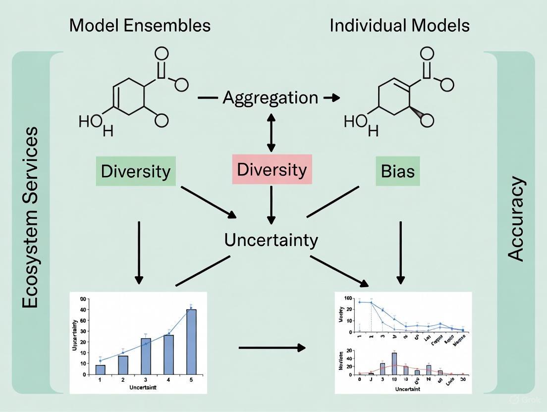
A study focusing on multiple ecosystem services across sub-Saharan Africa found that model ensembles were 5.0–6.1% more accurate than individual models [33]. The study also revealed that the variation among the constituent models within an ensemble (the ensemble's uncertainty) was negatively correlated with its accuracy. This means that the internal disagreement of an ensemble can serve as a useful proxy for its reliability, which is particularly valuable in data-deficient regions common in ES research [33].

Cross-Domain Experimental Evidence

The following table summarizes key performance metrics of ensemble methods from recent studies in various fields, illustrating their broad effectiveness.

Table 1: Comparative Performance of Ensemble Models Across Different Domains

Domain / Study	Top Performing Model(s)	Key Performance Metric	Reported Score	Comparison to Individual Models
Higher Education [6]	LightGBM (Boosting)	AUC	0.953	Outperformed other base learners and a stacking ensemble.
	Stacking Ensemble	AUC	0.835	Did not offer significant improvement over best base model.
Veterinary Medicine (LSD Prediction) [37]	Random Forest (Bagging) + ROS	Accuracy	82%	Superior performance among tested ensembles (DT, RF, AdaBoost, GBoost, XGBoost).
	XGBoost (Boosting)	Accuracy	81.25%	Competitive performance with Random Forest.
Heart Disease Prediction [39]	Ensemble (Bagging, Boosting, Stacking) with PCA/LDA	Accuracy	Up to 97%	Optimal accuracy, deemed well-suited for the method.
Pneumonia Classification [40]	VGG19/DenseNet121 + Random Forest	Accuracy	99.98%	Exemplifies hybrid DL/ML ensemble surpassing standalone deep learning models.

Key Comparative Insights

• Bagging vs. Boosting: While both are powerful, they excel in different scenarios. Bagging (e.g., Random Forest) is highly effective at reducing variance and is robust to overfitting. Boosting (e.g., XGBoost, LightGBM) often achieves lower bias and can yield higher accuracy on structured/tabular data, but may be more sensitive to noisy data [36] [37].
• The Stacking Paradox: While theoretically powerful, stacking does not always guarantee a significant performance improvement over a single well-tuned model, as seen in the higher education study where a stacking ensemble (AUC=0.835) was outperformed by a LightGBM base model (AUC=0.953) [6]. Its success heavily depends on the diversity and quality of the base models and the choice of an appropriate meta-learner.
• Overall Superiority: Despite nuances, a broad consensus exists that ensemble methods generally offer a significant performance boost. A large-scale comparison found that ensembles were 5.0–6.1% more accurate than individual models on average [33].

Detailed Experimental Protocols

To ensure the reproducibility and rigorous evaluation of ensemble models, researchers should adhere to structured experimental protocols. The following workflow outlines a comprehensive methodology applicable to ecosystem services research and other domains.

Diagram 2: Generalized Experimental Workflow for Ensemble Model Development. This protocol, synthesized from multiple studies, ensures robust model evaluation and is directly applicable to ecosystem services research [6] [37] [39].

Data Preparation and Class Imbalance

• Data Collection: In ES research, this often involves integrating multimodal data from diverse sources such as GIS databases, remote sensing imagery, field surveys, and climate models [6] [33].
• Addressing Class Imbalance: Many real-world ES datasets are imbalanced (e.g., rare species occurrences, specific land-use changes). Techniques to mitigate this include:
  • SMOTE (Synthetic Minority Over-sampling Technique): Generates synthetic samples for the minority class to balance the dataset [6] [37].
  • Random Oversampling (ROS): Randomly duplicates examples from the minority class [37].
  • Random Undersampling (RUS): Randomly removes examples from the majority class [37].
  • Studies show that combining ensemble methods with these techniques significantly improves prediction for minority classes [6] [37].

Model Training, Validation, and Interpretation

• Hyperparameter Tuning: Use methods like grid search or random search with cross-validation to optimize model parameters (e.g., n_estimators, learning_rate, max_depth for tree-based ensembles) [37]. This step enhances performance even on imbalanced data [37].
• Model Validation: Employ K-Fold Cross-Validation (e.g., 5-fold or 10-fold) to obtain reliable performance estimates and mitigate overfitting [6] [37]. Using stratified splits is crucial to maintain the class distribution in each fold.
• Model Interpretation and Fairness: For ES models to be actionable, they must be interpretable. SHAP (SHapley Additive exPlanations) analysis is widely used to identify the most influential predictors, ensuring model transparency [6] [37]. Furthermore, evaluating model fairness across different subpopulations (e.g., different regions or socio-economic groups) is critical, and techniques like SMOTE can also help improve fairness metrics [6].

This table details key computational tools and methodologies that function as the "research reagents" for developing and analyzing ensemble models in ecosystem services and related fields.

Table 2: Essential Computational Tools and Resources for Ensemble Learning Research

Tool / Resource	Type	Primary Function in Ensemble Research	Example Use Case
SMOTE [6] [37]	Algorithm	Addresses class imbalance by generating synthetic minority class samples.	Balancing a dataset of rare ecosystem service occurrences (e.g., specific pollination events) to improve model sensitivity.
SHAP [6] [37]	Analysis Framework	Provides post-hoc model interpretability by quantifying feature importance for individual predictions.	Identifying the most critical environmental drivers (e.g., precipitation, land cover) influencing carbon sequestration predictions.
Cross-Validation [6] [37]	Validation Protocol	Assesses model generalizability and robustness by rotating training and validation sets.	Providing a reliable estimate of how an ensemble model for water purification service will perform in unseen geographic regions.
Scikit-learn [36]	Python Library	Provides unified implementations of Bagging, Boosting, and Voting classifiers, and utilities for model evaluation.	Rapid prototyping and comparison of a Random Forest classifier against a Gradient Boosting classifier for habitat suitability modeling.
XGBoost / LightGBM [6] [36]	Software Library	Implements highly optimized gradient boosting algorithms, often achieving state-of-the-art results on tabular data.	Winning a predictive modeling competition for species distribution based on climatic and topographic variables.
Random Forest [36] [37]	Algorithm	A robust bagging ensemble that is less prone to overfitting and effective for high-dimensional data.	Initial baseline model for predicting the spread of invasive species, providing robust feature importance rankings.

The empirical evidence is clear: ensemble architectures consistently deliver more accurate, robust, and reliable predictive models compared to individual counterparts. In the specific context of ecosystem services research, where data can be complex, multimodal, and imbalanced, the adoption of ensemble methods is not just beneficial but necessary to advance the field [33].

While the "best" ensemble technique is context-dependent, bagging methods like Random Forest offer robust performance straight out of the box, whereas boosting methods like XGBoost and LightGBM often achieve top-tier accuracy at the cost of greater complexity and tuning. Stacking, while powerful, requires careful implementation to realize its theoretical advantages. As the field progresses, future work should focus on enhancing the interpretability and fairness of these ensemble black-box models and tailoring their objective functions to align directly with specific ecosystem management goals and cost-sensitive outcomes [34]. By integrating these advanced ensemble architectures, researchers and practitioners in ecosystem services can build more trustworthy tools to guide critical conservation and policy decisions.

In the pursuit of robust predictive models for critical fields like ecosystem services (ES) research and drug development, the debate between using individual models versus model ensembles is central. While complex, data-adaptive ensemble methods exist, this guide focuses on a comparison of two straightforward yet powerful techniques: unweighted averaging and median ensembles. These methods combine predictions from multiple models without requiring computationally intensive training of a meta-learner.

The core premise is that by aggregating predictions—either by simple averaging or by taking the median—the resulting ensemble can be more accurate and robust than any single constituent model. This guide objectively evaluates their performance against individual models and other ensemble alternatives across diverse scientific domains, providing experimental data and methodologies to inform researchers and drug development professionals.

Theoretical Foundation of Simple Ensembles

Core Concepts and Mechanisms

Ensemble learning operates on the principle that combining multiple models can mitigate the individual weaknesses and leverage the strengths of each, leading to improved overall performance. The two simple methods explored here are:

• Unweighted Averaging: This technique computes the arithmetic mean of the predicted values (for regression) or probabilities (for classification) from all base models in the library [41]. It effectively reduces variance without increasing bias, making it particularly useful when combining models of similar structure and performance [41] [42].
• Median Ensembles: This method uses the median of the predictions from all component models. The median is a robust location statistic that is less sensitive to extreme values or outliers than the mean, making the ensemble more resilient to occasional, severely misaligned predictions from one or more constituent models [43].

The effectiveness of these ensembles hinges on the concept of diversity among the base models. Ideally, different models should make errors on different parts of the input space so that they can cancel out each other's shortcomings [42].

The Bias-Variance Trade-off

The performance of a machine learning model can be decomposed into bias (error from erroneous assumptions) and variance (error from sensitivity to small fluctuations in the training data). A single complex model, like a deep neural network, often has low bias but high variance, leading to overfitting [41] [42].

Ensemble averaging addresses this dilemma. By combining multiple models, it reduces variance and improves generalization to unseen data, analogous to how financial portfolio diversification mitigates unsystematic risk [42]. The following diagram illustrates the workflow and core rationale behind using these simple ensembles.

Diagram 1: Workflow and rationale for unweighted averaging and median ensembles.

Experimental Evidence and Performance Comparison

Evidence from Ecosystem Services Research

In ES research, where model uncertainty is high and validation data are often scarce, ensemble approaches have proven their worth. A seminal study compared the accuracy of individual ES models against an ensemble for six different ecosystem services across sub-Saharan Africa [33] [44].

• Methodology: Multiple individual models were used to predict six ES. An unweighted ensemble was created by combining their predictions. The accuracy of both individual models and the ensemble was then evaluated against real validation data from the region [33].
• Results: The ensemble of models was a consistently better predictor than any single model. It demonstrated a 5.0–6.1% improvement in accuracy across the evaluated ecosystem services [33]. Furthermore, the variation among the constituent models within the ensemble was negatively correlated with its accuracy, providing a useful proxy for uncertainty in data-deficient areas [44].

Evidence from Public Health and Medical Applications

COVID-19 Forecasting

The U.S. COVID-19 Forecast Hub aggregated predictions from numerous teams to generate short-term burden forecasts. Researchers systematically studied ensemble methods to support public health decision-makers [43].

• Methodology: Researchers compared trained (weighted) ensembles with untrained, robust approaches. The key challenges addressed were occasional misalignment of forecasts with reported data and instability in the relative performance of forecasters over time [43].
• Results: In this unstable and high-stakes environment, an equally weighted median of all component forecasts emerged as a superior and robust choice. Its resilience to outlier predictions made it more reliable for policymakers than more complex, trained ensembles [43].

Hepatotoxicity Prediction

In drug development, predicting drug-induced liver injury is crucial. A 2024 study developed a comprehensive hepatotoxicity prediction model by integrating machine learning (ML) and deep learning (DL) algorithms [45].

• Methodology: After training individual base models on a large dataset of 2,588 chemicals using diverse molecular features, the study compared multiple ensemble strategies, including voting, bagging, and stacking [45].
• Results: The voting ensemble classifier, a form of weighted averaging, emerged as the optimal model. It achieved an accuracy of 80.26% and an AUC (Area Under the Curve) of 82.84%, outperforming other ensemble methods and individual models. It also showed high recall (over 93%), ensuring most hepatotoxic compounds were identified [45].

Evidence from Computer Vision and Cell Segmentation

A study on micrograph cell segmentation provides a direct comparison of averaging methods using deep convolutional neural networks (DCNNs) [46].

• Methodology: Ensembles were formed using the same VGG-style network architecture initialized with different random seeds and trained with variable numbers of examples. The performance of four averaging methods—mean, median, the location parameter of an alpha-stable distribution, and majority vote—was evaluated using accuracy and the Dice coefficient [46].
• Results: For this specific dataset, the choice of averaging method had only a marginal influence on the evaluation metrics. The study concluded that a simple mean was highly competitive with the most sophisticated methods and was the most proper ensemble method for this application due to its simplicity and speed [46].

Table 1: Quantitative performance comparison of ensemble methods across different fields.

Application Domain	Individual Model Performance	Unweighted Averaging Performance	Median Ensemble Performance	Key Finding
Ecosystem Services [33]	Baseline Accuracy	5.0-6.1% higher accuracy	Not Specifically Tested	Ensembles provide more accurate and robust estimates.
COVID-19 Forecasting [43]	Varies by contributor; unstable over time	Not the primary focus	Most robust choice for decision-making	Median outperformed trained ensembles in the presence of unstable component models.
Hepatotoxicity Prediction [45]	Baseline for comparison	Sub-optimal	Sub-optimal	Voting Ensemble (weighted) was optimal (80.26% Accuracy).
Cell Segmentation [46]	Baseline for comparison	Highly competitive (Accuracy & Dice)	Marginal difference from mean	Simplicity and speed of mean averaging make it the recommended choice.

Experimental Protocols for Key Studies

Protocol: Ecosystem Services Ensemble Modeling

The methodology for the ES study can be broken down into the following steps [33]:

• Model Selection: Gather multiple existing, independent modeling frameworks for the target ecosystem services (e.g., carbon sequestration, water flow).
• Prediction Generation: Run all models for the geographic area of interest (e.g., sub-Saharan Africa) to generate individual predictive maps for each ES.
• Ensemble Construction: For each location and ES, create an unweighted ensemble prediction by calculating the mean of all individual model outputs.
• Validation: Compare the predictions of individual models and the ensemble against a high-quality, observed validation dataset from the same region.
• Uncertainty Analysis: Calculate the variation (e.g., standard deviation) among the constituent model predictions at each location and correlate this with the ensemble's accuracy.

Protocol: COVID-19 Forecast Hub Ensemble

The CDC's approach for building a robust public health ensemble is as follows [43]:

• Data Aggregation: Collect forecasts (e.g., incident cases, deaths) from all contributing teams for the target period.
• Ensemble Formation:
  • Trained Ensemble: Use a statistical model to assign non-equal weights to contributors based on past performance.
  • Untrained Median Ensemble: Line up all forecasts for a given target and take the median value at each forecast horizon.
• Performance Monitoring: Continuously evaluate both ensemble types against subsequently reported data, with a focus on stability and reliability in the presence of component forecasters that may become misaligned or change in performance over time.
• Decision Support: Select the ensemble method that provides the most stable and reliable performance for use in official public health communications and policy.

Protocol: Micrograph Cell Segmentation Ensemble

The workflow for the image segmentation ensemble is visualized below [46]:

Diagram 2: Experimental workflow for the micrograph cell segmentation ensemble study.

The Scientist's Toolkit: Research Reagent Solutions

Table 2: Essential computational tools and their functions for implementing simple ensembles.

Tool / Solution	Function in Ensemble Research	Example Application
Scikit-Learn (Python)	Provides high-level implementations for easy prototyping of ensembles (e.g., VotingClassifier, VotingRegressor).	Rapidly ensemble Scikit-Learn models like Decision Trees, SVM, and KNN for a proof-of-concept study [42].
Deep Learning Frameworks (TensorFlow, PyTorch)	Train high-variance, low-bias base learners (e.g., Deep Neural Networks) and manually compute averaged/median predictions.	Implementing the averaging of multiple CNNs for image recognition tasks, as seen in ILSVRC challenges [41].
PyBioMed (Python Library)	Extracts a wide array of molecular descriptors and fingerprints from drug structures (SMILE) and protein sequences (FASTA).	Generating diverse feature sets for base models in a drug-target interaction (DTI) or hepatotoxicity prediction ensemble [47] [45].
RDKit (Cheminformatics Library)	Another robust toolkit for calculating molecular descriptors and manipulating chemical structures, often used in concert with ML.	Creating molecular fingerprints (e.g., Morgan fingerprints) as input features for models in a drug discovery ensemble [47].
Statistical Software (R, Python SciPy)	Calculates robust summary statistics, performs cross-validation, and conducts rigorous statistical tests to compare ensemble performance.	Computing the median of multiple forecast predictions for a robust ensemble, as in the COVID-19 Forecast Hub [43].

The body of experimental evidence confirms that simple ensemble methods are a powerful tool for improving predictive performance across diverse scientific fields. The choice between unweighted averaging and a median ensemble is context-dependent.

• Unweighted averaging is a strong default choice when combining models of similar type and performance, effectively reducing variance to boost accuracy, as seen in ecosystem services and image segmentation.
• Median ensembles shine in environments characterized by instability and potential for outlier predictions, such as the COVID-19 pandemic, providing superior robustness for decision-support systems.

For researchers in ecosystem services, drug development, and beyond, starting with these simple-to-implement ensembles provides a reliable baseline. They consistently outperform individual models and, in many cases, rival the performance of more complex, data-adaptive ensemble methods, all while offering greater transparency and computational efficiency.

Ensemble learning has emerged as a powerful methodology in machine learning, aggregating multiple learners to produce better predictive performance than any single constituent model. The technique rests on the foundational principle that a collectivity of learners yields greater overall accuracy than an individual learner [9]. In scientific research, particularly in domains requiring high-prediction reliability such as drug development and ecosystem services research, selecting appropriate strategies for combining these models becomes paramount. Advanced weighting strategies determine how each model's prediction contributes to the final ensemble output, fundamentally balancing the trade-offs between individual model excellence and collective consensus.

The core challenge in ensemble construction lies in the bias-variance tradeoff—managing the inverse relationship between a model's accuracy on training data (bias) and its performance on unseen data (variance) [9]. Ensemble methods strategically address this tradeoff by combining models with diverse characteristics. Weighting strategies operationalize this combination, primarily falling into two philosophical approaches: accuracy-based weighting that prioritizes historically superior performers, and consensus-driven approaches that leverage collective agreement, each with distinct mechanisms and optimal application scenarios. These approaches are not mutually exclusive but represent different points on a spectrum of how to value individual versus collective model intelligence.

Theoretical Foundations of Weighting Approaches

Accuracy-Based Weighting

Accuracy-based weighting operates on the principle of performance-driven selection, assigning influence to constituent models in direct proportion to their historical predictive accuracy. This approach implicitly assumes that models demonstrating superior performance on validation or training datasets will maintain that superiority in production environments. The implementation typically involves quantifying model performance using metrics such as accuracy, AUC (Area Under the Curve), F1-score, or log loss, then normalizing these metrics to generate weights that sum to unity across the ensemble [5].

The mathematical foundation for accuracy-based weighting often draws from Bayesian model averaging or performance-weighted linear combinations. In practice, weights ((wi)) for each model (i) might be calculated using softmax transformation of performance scores: (wi = \frac{\exp(\beta \cdot si)}{\sumj \exp(\beta \cdot sj)}), where (si) is the performance score of model (i) and (\beta) is a temperature parameter controlling how strongly weights concentrate on the top performers. This approach creates a performance hierarchy within the ensemble, where consistently accurate models dominate the final prediction.

Consensus-Driven Approaches

Consensus-driven weighting prioritizes collective agreement over individual excellence, operating on the sociological principle that diverse independent judgments often yield more robust decisions than expert-driven hierarchies. These methods include straightforward majority voting, weighted voting based on model confidence estimates, and more sophisticated entropy-based methods that prioritize models when they exhibit high confidence in their predictions [48] [9].

Unlike accuracy-based methods that require historical performance data, pure consensus approaches like majority voting are data-agnostic, making them particularly valuable in scenarios with limited validation data or non-stationary data distributions where past performance may not reliably indicate future success. The theoretical justification stems from the Condorcet jury theorem, which mathematically demonstrates that under certain conditions, the probability of a correct collective decision approaches 1 as the number of voters increases, even when individual voters are only marginally competent. Intermediate approaches incorporate confidence scores through methods like Bayesian model combination or stacking with meta-learners that optimize the consensus function [9] [49].

Comparative Analysis of Ensemble Weighting Strategies

Performance Comparison Across Domains

Table 1: Performance Comparison of Ensemble Weighting Strategies in Educational Forecasting

Ensemble Strategy	Base Models	Performance Metric	Score	Application Context
LightGBM (Accuracy-Weighted)	Gradient Boosting	AUC	0.953	Student Performance Prediction [6]
Stacking Ensemble	Multiple Heterogeneous	AUC	0.835	Student Performance Prediction [6]
Gradient Boosting	Decision Trees	Global Accuracy (Macro)	67%	Multiclass Grade Prediction [5]
Random Forest	Decision Trees (Bagging)	Global Accuracy (Macro)	64%	Multiclass Grade Prediction [5]
Bagging	Decision Trees	Global Accuracy (Macro)	65%	Multiclass Grade Prediction [5]
Support Vector Machine	N/A	Micro Prediction Accuracy	19%	Individual Student Grade [5]
XGBoost	Decision Trees (Boosting)	Micro Prediction Accuracy	33%	Individual Student Grade [5]
Random Forest	Decision Trees	Micro Prediction Accuracy	22%	Individual Student Grade [5]

Table 2: Computational Performance of Bagging vs. Boosting

Ensemble Method	Ensemble Complexity	Performance (MNIST)	Computational Time	Performance Trend
Bagging	20 base learners	0.932	Reference (1x)	Diminishing returns with complexity [17]
Bagging	200 base learners	0.933	~Linear increase	Performance plateaus [17]
Boosting	20 base learners	0.930	~7x Bagging	Rapid initial improvement [17]
Boosting	200 base learners	0.961	~14x Bagging	Potential overfitting at high complexity [17]

The comparative data reveals several critical patterns. In educational forecasting applications, accuracy-based boosting methods like LightGBM demonstrate superior performance with an AUC of 0.953, significantly outperforming stacking ensembles which achieved only 0.835 AUC in the same study [6]. This superiority comes despite stacking's theoretical advantage of leveraging heterogeneous models through a meta-learner. Similarly, for multiclass grade prediction, gradient boosting achieved the highest global macro accuracy at 67%, followed closely by bagging at 65% and random forests at 64% [5].

However, the performance hierarchy shifts when considering micro-level prediction accuracy for individual students. In this context, XGBoost achieved 33% accuracy, substantially outperforming random forests (22%) and support vector machines (19%) [5]. This divergence highlights a crucial consideration: the optimal weighting strategy depends fundamentally on the prediction granularity and performance metric employed. For institutional-level interventions where overall accuracy matters most, accuracy-weighted boosting methods appear superior, while for individual student interventions, the best approach may vary significantly.

Computational efficiency represents another critical differentiator. As shown in Table 2, bagging exhibits nearly linear computational scaling with ensemble complexity, with performance plateauing as more base learners are added. In contrast, boosting demonstrates dramatically higher computational requirements—approximately 14 times greater than bagging at 200 base learners—but delivers continuous performance improvements, eventually surpassing bagging's capabilities, though with risks of overfitting at high complexity levels [17]. This creates a clear tradeoff: practitioners prioritizing computational efficiency may prefer bagging, while those prioritizing predictive accuracy may opt for boosting despite its higher computational cost [17].

Contextual Advantages and Limitations

Table 3: Situational Advantages of Ensemble Weighting Strategies

Application Scenario	Recommended Approach	Rationale	Key Evidence
High Signal-to-Noise Data	Accuracy-Based Weighting	Superior models consistently outperform	LightGBM achieving 0.953 AUC [6]
Resource-Constrained Environments	Bagging with Simple Voting	Better computational efficiency	Bagging requiring 14x less computation than boosting [17]
Heterogeneous Data Distributions	Consensus-Driven with Routing	Specialized models for different data regions	Hellsemble's "circles of difficulty" approach [48]
Unstable Performance Patterns	Dynamic Ensemble Selection	Adapts to local instance characteristics	DES methods selecting competent models per instance [48]
Multiclass Imbalanced Targets	Gradient Boosting	Handles complex class structures	67% macro accuracy vs. 64% for random forest [5]
Requirement for Interpretability	Consensus-Driven Methods	More transparent decision pathways	Router-based approaches providing clearer specialization [48]

Accuracy-based weighting strategies, particularly those implemented through boosting algorithms, generally deliver superior predictive performance in environments with stable data distributions and clear performance differentials between models. As evidenced by multiple studies [6] [5], boosting techniques like LightGBM and XGBoost consistently achieve top rankings across various metrics. However, this performance advantage comes with substantial computational overhead and increased risk of overfitting when ensemble complexity becomes excessive [17]. The diminishing returns observed with bagging as ensemble size increases appears much less pronounced with boosting, though careful monitoring is essential to prevent performance degradation from over-specialization.

Consensus-driven approaches offer distinct advantages in scenarios involving heterogeneous data distributions or specialized model capabilities. The Hellsemble framework exemplifies this approach, incrementally partitioning datasets into "circles of difficulty" and routing instances to specialized models [48]. This strategy mimics human expert panels where different specialists address problems matching their expertise. Similarly, dynamic ensemble selection (DES) methods maintain a pool of models but select the most competent subset for each specific instance based on local performance estimates [48]. These approaches demonstrate particular value when dealing with non-stationary data or when interpretability requirements favor more transparent specialization patterns.

Experimental Protocols and Methodologies

Benchmarking Ensemble Performance

Robust evaluation of ensemble weighting strategies requires meticulous experimental design to ensure fair comparisons and generalizable findings. The methodology employed by [6] provides an exemplary protocol for benchmarking ensemble performance:

• Data Preparation and Feature Selection: Collect and integrate multimodal data sources (LMS interactions, academic history, demographics). Perform data cleaning and standardization. Select features based on literature review and ethical considerations— [6] utilized 22 features across three categories: academic performance indicators, VLE interaction metrics, and demographic characteristics.

• Class Balancing: Address class imbalance using techniques like SMOTE (Synthetic Minority Over-sampling Technique), particularly crucial when predicting at-risk populations where minority classes are often of primary interest [6].

• Model Training and Validation: Implement multiple base learners (traditional algorithms, Random Forest, gradient boosting variants) alongside ensemble combinations. Employ 5-fold stratified cross-validation to ensure robust performance estimation and mitigate overfitting [6].

• Performance Assessment: Evaluate models using multiple metrics including AUC, F1-score, precision, and recall. Additionally, assess fairness across demographic subgroups using metrics like consistency ratio (with ideal being 1.0) [6].

• Interpretability Analysis: Apply techniques like SHAP (SHapley Additive exPlanations) to identify influential predictors and validate model logic against domain knowledge [6].

This comprehensive protocol ensures that performance comparisons reflect true methodological differences rather than experimental artifacts.

Computational Efficiency Evaluation

The methodology from [17] provides a rigorous framework for evaluating computational aspects:

• Theoretical Modeling: Develop mathematical models hypothesizing relationships between ensemble complexity (number of base learners) and algorithm performance for both bagging and boosting approaches.

• Experimental Validation: Test theoretical models across multiple datasets (MNIST, CIFAR-10, CIFAR-100, IMDB) with varying complexity characteristics and computational environments.

• Performance Profiling: Measure algorithm performance (accuracy) alongside computational costs (time, resources) across a range of ensemble complexities.

• Tradeoff Analysis: Define "algorithmic profit" incorporating both performance and cost dimensions based on decision-maker preferences, identifying optimal operating points for each method.

This methodology enables practitioners to select ensemble strategies based not merely on raw performance but on efficiency considerations relevant to resource-constrained environments.

Visualization of Ensemble Weighting Strategies

Ensemble Weighting Strategy Selection Workflow

The visualization illustrates the conceptual workflow for implementing advanced weighting strategies in ensemble learning. The process begins with input data flowing to multiple base models trained in parallel. The critical decision point emerges after model training, where practitioners must select between accuracy-based and consensus-driven weighting approaches. Accuracy-based weighting incorporates historical performance data and validation metrics to compute model-specific weights, resulting in weighted averaging for final predictions. Conversely, consensus-driven approaches employ majority voting mechanisms that prioritize agreement over individual excellence. This branching pathway highlights the fundamental methodological choice confronting ensemble designers.

Research Reagent Solutions for Ensemble Experiments

Table 4: Essential Research Components for Ensemble Learning Experiments

Research Component	Function	Example Implementations
Base Learning Algorithms	Foundation models for ensemble construction	Decision Trees, SVM, K-Nearest Neighbors [5]
Ensemble Frameworks	Implementation of weighting strategies	Random Forest (Bagging), XGBoost (Boosting) [6] [5]
Performance Metrics	Quantification of model performance	AUC, F1-Score, Precision, Recall, Macro/Micro Accuracy [6] [5]
Validation Methodologies	Robust performance estimation	5-fold Stratified Cross-Validation [6]
Interpretability Tools	Model explanation and validation	SHAP (SHapley Additive exPlanations) [6]
Computational Resources	Handling resource-intensive training	High-performance computing for boosting ensembles [17]

Successful implementation of advanced weighting strategies requires careful selection of methodological components. Base learning algorithms form the foundational elements, with diverse algorithms (decision trees, SVM, K-nearest neighbors) recommended to create complementary strengths within the ensemble [5]. Ensemble frameworks operationalize the weighting strategies, with popular implementations including Random Forest for bagging, XGBoost and LightGBM for boosting, and stacking ensembles for meta-learning approaches [6] [5].

Performance metrics must be carefully selected to align with research objectives, with AUC and F1-score particularly valuable for imbalanced classification problems common in scientific applications [6]. The distinction between macro and micro accuracy metrics can reveal important performance patterns across different prediction granularities [5]. Validation methodologies like 5-fold stratified cross-validation provide robust performance estimation while mitigating overfitting [6]. For interpretability, SHAP analysis offers consistent model explanations and validates that influential predictors align with domain knowledge [6]. Finally, adequate computational resources are essential, particularly for boosting ensembles which can require 14 times more computational time than bagging approaches at similar complexity levels [17].

The comparative analysis of advanced weighting strategies reveals a nuanced landscape where no single approach dominates across all scenarios. Accuracy-based weighting strategies, particularly those implemented through boosting algorithms like LightGBM and XGBoost, generally deliver superior predictive performance in environments with stable data distributions and adequate computational resources [6] [5]. These methods excel when clear performance differentials exist between models and when prediction accuracy outweighs computational efficiency concerns.

Conversely, consensus-driven approaches offer compelling advantages in scenarios featuring heterogeneous data distributions, specialized model capabilities, or stringent interpretability requirements [48]. Methods like dynamic ensemble selection and router-based frameworks provide adaptive mechanisms for handling data complexity while maintaining transparent decision pathways. The computational efficiency of bagging-based consensus methods makes them particularly valuable in resource-constrained environments [17].

For research applications in domains such as drug development and ecosystem services, the selection between accuracy-based and consensus-driven approaches must consider contextual requirements including data characteristics, computational constraints, interpretability needs, and performance objectives. Hybrid frameworks that strategically combine elements of both approaches represent a promising direction for future methodology development, potentially offering robust performance across diverse application contexts while balancing the competing demands of accuracy, efficiency, and interpretability.

Ensemble learning represents a powerful meta-technique in machine learning that aggregates predictions from multiple base models to produce a single, superior predictive output. This approach operates on the core principle that a collectivity of learners yields greater overall accuracy than an individual learner, effectively harnessing the "wisdom of crowds" phenomenon [9] [50]. The fundamental principles underpinning successful ensemble methods include diversity (base models must differ from each other to produce different errors), independence (models should train independently where possible), and intelligent aggregation (the method of combining predictions must be optimized) [50].

In the context of model ensembles versus individual model accuracy, ensemble methods strategically address the classic bias-variance tradeoff that plagues individual models. Bias measures the average difference between predicted values and true values, while variance measures the difference between predictions across various realizations of a given model [9]. Ensemble learning techniques can effectively reduce both bias and variance, whereas individual models typically struggle to optimize both simultaneously. By combining multiple models, ensemble approaches achieve a more favorable balance in this tradeoff, leading to enhanced generalization performance and more robust predictions across various domains, including pharmaceutical research, healthcare diagnostics, and educational analytics [51] [18] [6].

The ecosystem of ensemble methods primarily encompasses three major paradigms: bagging (Bootstrap Aggregating), boosting, and stacking. Each employs distinct mechanisms for combining models: bagging operates through parallel training of homogeneous models on different data subsets, boosting functions via sequential training with error correction, and stacking utilizes a meta-learner to optimally combine predictions from heterogeneous base models [9] [50]. This guide provides a comprehensive comparison of how these ensemble strategies, particularly those leveraging Random Forests (RF), XGBoost, and Neural Networks, perform against individual models and each other across diverse experimental settings and application domains.

Ensemble Methodologies: Technical Foundations

Bagging and Random Forest

Bagging (Bootstrap Aggregating) is a homogeneous parallel ensemble method that creates multiple versions of the training data through bootstrap resampling (random sampling with replacement) and trains a base model on each of these versions [9]. The final prediction is generated by aggregating the predictions of all base models, typically through majority voting for classification problems or averaging for regression tasks. This approach particularly effective at reducing variance and mitigating overfitting, especially when applied to high-variance models like decision trees [50].

Random Forest extends the bagging concept by incorporating feature randomness along with data randomness. While standard bagging samples every feature to identify the best split, Random Forest iteratively samples random subsets of features to create decision nodes [9]. This additional layer of randomness further decorrelates the individual trees, resulting in improved generalization and robust performance. Random Forest ensembles are particularly valued for their high stability, parallelizable training process, and reduced sensitivity to hyperparameter tuning [50].

Boosting and XGBoost

Boosting represents a sequential ensemble approach where models are trained in a chain, with each subsequent model focusing on correcting the errors of its predecessors [9]. Unlike bagging, which combines independent models, boosting creates a strong learner by iteratively adding weak learners that concentrate on previously misclassified examples. The fundamental principle involves weighting misclassified instances more heavily in subsequent training iterations, allowing the algorithm to progressively focus on harder-to-predict cases [50].

XGBoost (Extreme Gradient Boosting) is an optimized implementation of gradient boosting that incorporates advanced features including regularization terms to control model complexity, parallel processing for computational efficiency, and sophisticated handling of missing values [50]. Instead of simply weighting misclassified samples, XGBoost uses gradient descent to minimize a loss function by adding trees that predict the residuals or negative gradients of previous models. This approach has demonstrated exceptional performance across numerous machine learning competitions and real-world applications, often achieving state-of-the-art results on structured data problems [6] [52].

Stacking and Neural Network Integration

Stacking (Stacked Generalization) employs a heterogeneous parallel approach where multiple different base models (e.g., Random Forest, XGBoost, Neural Networks) are trained on the same dataset, and their predictions are then used as input features for a meta-learner that learns how to best combine them [9] [50]. This two-layer structure allows stacking to leverage the unique strengths of diverse modeling approaches, with the meta-model learning which base models to trust more heavily under specific data conditions.

Neural Networks can serve as both powerful base models within ensembles and as meta-learners in stacking frameworks. Their capacity to model complex non-linear relationships makes them particularly valuable in heterogeneous ensembles [50]. In the context of stacking, neural networks can function as meta-learners that capture intricate patterns in the relationship between base model predictions and the true target variable, potentially discovering nuanced combination strategies that simpler linear models might miss [6] [53].

Workflow Diagram of Ensemble Methods

The following diagram illustrates the general workflow and logical relationships between the major ensemble learning methods:

Ensemble Learning Workflow

Comparative Performance Analysis

Experimental Data from Multiple Domains

Recent research across diverse domains provides compelling evidence for the performance advantages of ensemble methods compared to individual models. The following table summarizes key experimental findings:

Table 1: Performance Comparison of Ensemble Methods Across Domains

Application Domain	Best Performing Model	Key Performance Metrics	Comparison Models	Reference
Colorectal Cancer Classification	Random Forest	F1-score: 0.93, Minimal misclassifications	XGBoost (F1: 0.92), SVM, DNN	[51]
Academic Performance Prediction	LightGBM	AUC: 0.953, F1: 0.950	Stacking (AUC: 0.835), Random Forest, XGBoost	[6]
Network Intrusion Detection	Random Forest	Accuracy: 99.80%	XGBoost, Deep Neural Networks	[54]
Vehicle Traffic Prediction	XGBoost	Superior MAE and MSE values	RNN-LSTM, SVM, Random Forest	[52]
Drug Solubility Prediction	Voting Ensemble (MLP + GPR)	Superior accuracy vs. individual models	MLP, GPR (individual)	[53]

The consistent outperformance of ensemble methods across these diverse applications demonstrates their robustness and generalizability. In colorectal cancer classification using exome datasets, both Random Forest and XGBoost achieved exceptional F1-scores (0.93 and 0.92 respectively), significantly outperforming individual Support Vector Machines and Deep Neural Networks which showed low accuracy and were not pursued further in the study [51]. Similarly, in network security, Random Forest achieved remarkable 99.80% accuracy in intrusion detection, surpassing both XGBoost and Deep Neural Networks when optimized with SMOTE for handling class imbalance and Optuna for hyperparameter tuning [54].

Domain-Specific Performance Patterns

Different ensemble methods exhibit distinct advantages across problem domains. For educational analytics predicting student academic performance, gradient boosting methods (LightGBM and XGBoost) demonstrated superior performance compared to bagging approaches, with LightGBM achieving an AUC of 0.953 and F1-score of 0.950 [6]. Interestingly, in this application, a stacking ensemble did not offer significant performance improvement over the best individual model (LightGBM) and showed considerable instability, suggesting that added complexity doesn't always guarantee better results [6].

In time series forecasting with highly stationary data, such as predicting vehicle traffic through Italian tollbooths, XGBoost outperformed both Random Forest and deep learning models (RNN-LSTM), particularly in terms of MAE (Mean Absolute Error) and MSE (Mean Squared Error) metrics [52]. This demonstrates that ensemble methods can sometimes surpass more complex deep learning approaches, especially when dealing with specific data characteristics like high stationarity.

For pharmaceutical research predicting drug solubility in supercritical solvents for continuous manufacturing, a voting ensemble combining Gaussian Process Regression (GPR) and Multi-layer Perceptron (MLP) networks demonstrated superior accuracy compared to either individual model [53]. This hybrid approach leveraged the strengths of both probabilistic modeling (GPR) and neural networks (MLP), optimized using Grey Wolf Optimization (GWO) for hyperparameter tuning.

Detailed Experimental Protocols

Colorectal Cancer Classification Protocol

The experimental protocol for colorectal cancer classification exemplifies a rigorous approach to biomedical ensemble modeling:

Data Source and Preprocessing: Publicly available CRC exome datasets from NCBI SRA were analyzed using a custom-built automated NGS pipeline. Feature engineering was performed to select relevant genomic variants, focusing on identifying potential biomarkers for improved diagnosis and personalized treatment strategies [51].

Model Training and Validation: Multiple ML algorithms were employed for model building, including Random Forest and XGBoost. Model performance was evaluated using comprehensive metrics including F1-scores, ROC curves, and precision-recall curves. The models were validated using appropriate cross-validation techniques to ensure generalizability [51].

Deployment: The best-performing models were integrated into a web application deployed on Posit Connect Cloud through Shiny Python, providing a valuable resource for the CRC community and facilitating streamlined analysis and improved decision-making [51].

Educational Analytics Experimental Framework

The methodology for predicting academic performance showcases ensemble applications in social sciences:

Data Collection and Feature Engineering: Data from 2,225 engineering students was collected through an ETL process from Moodle Virtual Learning Environment and academic records. Features were categorized into three main types: academic performance indicators (previous grades, exam scores), VLE interaction metrics (assignments reviewed, course accesses, quizzes completed), and demographic data [6].

Class Balancing and Validation: SMOTE (Synthetic Minority Oversampling Technique) was applied to address class imbalances. The study employed a comparative evaluation of seven base learners using 5-fold stratified cross-validation, including traditional algorithms, Random Forest, and gradient boosting ensembles (XGBoost, LightGBM), and a final stacking model [6].

Fairness and Interpretability Analysis: Beyond standard performance metrics, the study conducted comprehensive fairness evaluations across gender, ethnicity, and socioeconomic status (achieving consistency = 0.907) and model interpretability analysis using SHAP (SHapley Additive exPlanations) to identify the most influential predictors [6].

Stacking Ensemble Methodology

The following diagram illustrates the architectural framework of stacking ensembles, which combines predictions from multiple base models using a meta-learner:

Stacking Ensemble Architecture

The Researcher's Toolkit: Essential Materials and Methods

Table 2: Essential Research Reagents and Computational Tools for Ensemble Experiments

Tool/Technique	Category	Function in Ensemble Research	Example Implementation
SMOTE	Data Preprocessing	Addresses class imbalance by generating synthetic minority class samples	Improved recall for minority classes in educational analytics [6] and intrusion detection [54]
SHAP Analysis	Model Interpretability	Explains model predictions by quantifying feature importance	Identified early grades as most influential predictors in student performance models [6]
Optuna	Hyperparameter Optimization	Automates hyperparameter tuning for optimal model performance	Used with Random Forest to achieve 99.80% accuracy in intrusion detection [54]
Cross-Validation	Model Validation	Provides robust performance estimation while mitigating overfitting	5-fold stratified cross-validation in educational analytics [6]
Grey Wolf Optimization	Metaheuristic Optimization	Optimizes hyperparameters for ensemble models in complex spaces	Tuned voting ensemble for drug solubility prediction [53]
ROC Curves	Model Evaluation	Visualizes classification performance across different thresholds	Evaluated CRC classification models [51]
Voting/Averaging	Prediction Aggregation	Combines predictions from multiple base models	Simple yet effective aggregation in bagging and boosting ensembles [9]

The comprehensive comparison of ensemble methods presented in this guide demonstrates their consistent superiority over individual models across diverse application domains, from healthcare and pharmaceuticals to education and cybersecurity. The experimental evidence confirms that ensemble methods—particularly Random Forest, XGBoost, and strategically designed stacking ensembles—typically deliver enhanced predictive accuracy, improved generalization, and greater robustness compared to individual models.

The strategic selection of ensemble methodologies should be guided by specific problem characteristics: Random Forest excels in scenarios requiring robust performance with minimal hyperparameter tuning, XGBoost often achieves state-of-the-art results on structured data problems, and stacking ensembles provide maximum flexibility for leveraging diverse modeling approaches through meta-learning. However, the added complexity of stacking does not always guarantee performance improvements, as evidenced by the educational analytics case where a well-tuned LightGBM model outperformed a stacking ensemble [6].

For researchers and practitioners in model-informed drug development and other scientific domains, ensemble methods offer powerful tools for enhancing decision-making through improved predictive accuracy [18]. As the field evolves, the integration of ensemble methods with emerging technologies like explainable AI and automated machine learning will further expand their utility and application across the research ecosystem.

Optimizing Water Quality Management in Tilapia Aquaculture

The optimization of water quality management is a cornerstone for the success and sustainability of tilapia aquaculture, a critical sector for global food security. Traditional approaches to monitoring and managing complex water parameters have relied on individual predictive models or manual assessment, but these methods often face limitations in accuracy, robustness, and generalizability across diverse aquaculture environments. Recent advancements in machine learning (ML) and modeling approaches present an opportunity to transform water quality management through data-driven decision support systems. This comparison guide examines a paradigm shift occurring across environmental sciences: the movement from relying on single models toward employing model ensembles that aggregate predictions from multiple algorithms. This approach, validated extensively in ecosystem services research, demonstrates that ensembles provide 5.0–6.1% greater accuracy on average compared to individual models while simultaneously providing valuable uncertainty estimates [33] [44].

The application of ensemble modeling to tilapia aquaculture represents a promising frontier for improving operational decisions. By leveraging multiple machine learning algorithms working in concert—including Random Forest, Gradient Boosting, Neural Networks, and ensemble classifiers—aquaculture operators can achieve more reliable predictions of optimal management actions based on key environmental parameters. This guide systematically compares the performance of individual versus ensemble modeling approaches, provides detailed experimental methodologies from current research, and offers practical implementation frameworks for integrating these advanced analytical techniques into tilapia aquaculture operations.

Performance Comparison: Individual vs. Ensemble Models

Quantitative Performance Metrics in Aquaculture Applications

Recent research directly applicable to tilapia aquaculture has demonstrated that multiple machine learning models can achieve exceptional performance in predicting optimal water quality management decisions. A 2025 study developing decision-support systems for tilapia aquaculture evaluated several algorithms on a synthetic dataset representing 20 critical water quality scenarios, with results showing that multiple individual models including Random Forest, Gradient Boosting, XGBoost, and Neural Networks all achieved perfect accuracy (100%) on held-out test data when predicting optimal management actions [55].

Table 1: Performance Comparison of Machine Learning Models in Tilapia Aquaculture

Model Type	Accuracy (%)	Precision	Recall	F1-Score	Cross-Validation Stability
Voting Classifier (Ensemble)	100.0	Perfect	Perfect	Perfect	High
Random Forest	100.0	Perfect	Perfect	Perfect	High
Gradient Boosting	100.0	Perfect	Perfect	Perfect	High
XGBoost	100.0	Perfect	Perfect	Perfect	High
Neural Network	100.0	Perfect	Perfect	Perfect	Highest (98.99% ± 1.64%)
Support Vector Machines	Lower than above	Not specified	Not specified	Not specified	Not specified
Logistic Regression	Lower than above	Not specified	Not specified	Not specified	Not specified

While these results might suggest equivalence between individual and ensemble approaches, cross-validation revealed important differences in model stability. The Neural Network achieved the highest mean cross-validation accuracy at 98.99% ± 1.64%, indicating remarkable consistency across different data partitions [55]. This suggests that model selection should be guided by specific deployment requirements rather than test accuracy alone, with each approach offering distinct advantages for different operational priorities.

Ecosystem Services Research: Evidence for Ensemble Superiority

Research from ecosystem services (ES) modeling provides compelling evidence for the ensemble approach that can be extrapolated to aquaculture applications. Across six different ecosystem services in sub-Saharan Africa, ensemble modeling consistently outperformed individual models, demonstrating 5.0–6.1% greater accuracy on average [33] [44]. This performance advantage held across diverse environmental contexts and modeling challenges.

Table 2: Ensemble Model Performance Advantages in Environmental Applications

Application Domain	Accuracy Improvement	Uncertainty Quantification	Geographic Robustness	Data Efficiency
Ecosystem Services (General)	5.0–6.1% higher than individual models	Built-in through model variation	More consistent across regions	Effective even in data-poor regions
Global ES Ensembles	2–14% more accurate than individual models	Yes, via variation among models	High global consistency	Reduces capacity gaps in poorer regions
Tilapia Aquaculture ML	Multiple perfect scores but varying stability	Not explicitly measured	Not tested	Works with synthetic data

A critical advantage of ensemble approaches identified in ES research is their ability to provide inherent uncertainty quantification. The variation among constituent models within an ensemble negatively correlates with accuracy, providing a valuable proxy for confidence estimates when validation data are unavailable [44]. This feature is particularly valuable for aquaculture operations in data-deficient areas or when developing future scenarios.

Experimental Protocols and Methodologies

Water Quality Management Decision Support Protocol

The experimental methodology for developing ML-based water quality management systems in tilapia aquaculture involves several carefully designed stages, as implemented in a recent study achieving exceptional prediction accuracy [55]:

Dataset Generation and Preprocessing:

• Synthetic dataset creation representing 20 critical water quality scenarios in tilapia aquaculture
• Class balancing using SMOTETomek algorithm to address potential imbalance in management decision classes
• Feature scaling to normalize the range of input water quality parameters
• Parameter inclusion: Comprehensive water quality metrics (temperature, dissolved oxygen, pH, ammonia, nitrite, alkalinity, transparency)

Model Development and Training:

• Algorithm selection: Random Forest, Gradient Boosting, XGBoost, Support Vector Machines, Logistic Regression, Neural Networks
• Ensemble method: Voting Classifier combining predictions from multiple base models
• Training paradigm: Supervised learning with historical water quality parameters as features and expert management decisions as labels
• Validation approach: k-fold cross-validation to ensure robustness and prevent overfitting

Performance Evaluation:

• Primary metrics: Accuracy, precision, recall, F1-score
• Cross-validation consistency assessment
• Computational efficiency analysis for real-time deployment potential

This protocol resulted in the development of a decision-support system that moves beyond simple parameter prediction to automating management decisions, representing a significant advancement in operational intelligence for aquaculture operations [55].

Biofloc System Optimization Protocol

Complementing the ML approach, research into biofloc technology (BFT) systems provides additional methodology for water quality optimization in tilapia aquaculture, particularly relevant for systems utilizing varying water salinities [56]:

Experimental Design:

• Four BFT treatments with varying salinity levels (0 ppt, 12 ppt, 24 ppt, 36 ppt)
• Triplicate experimental setup using 12 fiberglass tanks (250 L each)
• Florida red tilapia fry (average initial weight: 1.73 ± 0.01 g/fish)
• 75-day experimental duration

Biofloc System Initiation:

• Carbon/nitrogen ratio maintenance at 15:1 using rice bran as carbon source
• Initial biofloc development in fiberglass jars with dechlorinated water
• Continuous aeration and agitation for microbial activity maintenance
• Regular monitoring of floc development and microbial communities

Data Collection and Analysis:

• Water quality parameters: ammonia, nitrite, dissolved oxygen, pH, alkalinity
• Growth metrics: final weight, weight gain, specific growth rate
• Physiological indicators: immune response (IgM), stress parameters (cortisol)
• Histopathological analysis: liver and intestinal health
• Pathogenic bacterial load counts

This methodology identified that 12-24 ppt salinity in BFT systems optimized growth performance, immune response, and water quality for Florida red tilapia, demonstrating how environmental parameter optimization can enhance productivity [56].

Visualization of Model Ensemble Framework

Ensemble Modeling Framework for Aquaculture

Research Reagent Solutions and Essential Materials

Table 3: Essential Research Materials for Aquaculture ML and Biofloc Experiments

Category	Specific Materials/Reagents	Function/Application	Experimental Context
ML Data Processing	SMOTETomek Algorithm	Class balancing for imbalanced decision datasets	Preprocessing synthetic water quality scenario data [55]
ML Algorithms	Random Forest, Gradient Boosting, XGBoost, Neural Networks	Base predictive models for management decisions	Individual model development [55]
Ensemble Methods	Voting Classifier	Combining predictions from multiple models	Final decision support system [55]
Biofloc Components	Rice Bran	Carbon source for maintaining C/N ratio (15:1)	Biofloc system initiation and maintenance [56]
Water Analysis	Test kits for ammonia, nitrite, pH, dissolved oxygen, alkalinity	Monitoring critical water quality parameters	Both ML validation and biofloc optimization [55] [56]
Salinity Adjustment	Underground saline water (USW), Dechlorinated freshwater	Creating specific salinity conditions (0, 12, 24, 36 ppt)	Salinity optimization experiments [56]

The evidence from both aquaculture-specific machine learning applications and broader ecosystem services research consistently demonstrates the superiority of ensemble modeling approaches over reliance on individual algorithms. While individual models can achieve perfect accuracy under specific test conditions, ensembles provide greater robustness, uncertainty quantification, and consistent performance across varying conditions—critical attributes for real-world aquaculture operations where environmental conditions constantly fluctuate.

For researchers and aquaculture professionals implementing these approaches, we recommend:

• Prioritize ensemble approaches for operational decision support systems, leveraging the documented 5.0-6.1% accuracy advantage observed in ecosystem services research [33] [44]
• Combine ML approaches with proven biotechnologies like biofloc systems that naturally enhance water quality while providing additional nutritional sources [56]
• Implement comprehensive monitoring regimes tracking both water quality parameters and fish health indicators to continuously refine model accuracy
• Select modeling approaches based on deployment context rather than test accuracy alone, considering computational requirements, interpretability needs, and integration capabilities with existing farm management systems

The integration of ensemble modeling approaches with sustainable aquaculture technologies represents a promising pathway toward more productive, efficient, and environmentally responsible tilapia production systems capable of meeting growing global protein demands while minimizing ecological impacts.

Overcoming Computational and Practical Hurdles in Ensemble Deployment

In the rapidly evolving fields of machine learning and scientific research, particularly in computationally intensive domains like drug discovery, a persistent assumption has taken root: that ensemble models, while often more accurate, invariably demand greater computational resources than single-model approaches. This perception has sometimes limited their adoption in resource-constrained environments. However, a growing body of evidence from cutting-edge research challenges this cost myth, demonstrating that strategically designed ensembles can in fact provide a faster, more efficient path to high accuracy. This guide objectively compares the performance of ensemble methods against individual models, presenting quantitative data and experimental protocols that reveal how ensembles achieve superior performance while managing—and in some cases, significantly reducing—computational costs. By framing this analysis within the broader context of model accuracy ecosystem services, we explore how ensembles contribute robust, efficient, and scalable predictive capabilities that benefit scientific applications from pharmaceutical development to educational analytics.

Theoretical Foundations: How Ensembles Achieve More with Less

Ensemble learning operates on the principle that combining multiple models can produce better performance than any single constituent model. The efficiency gains are achieved through several mechanisms. Bagging (Bootstrap Aggregating) reduces variance and overfitting by training multiple versions of a model on different random subsets of the training data [57] [17]. Boosting sequentially trains models, with each new model focusing on the errors of its predecessors, thereby reducing bias [57] [17]. Stacking combines multiple models using a meta-learner that learns how to best weight their predictions [6] [57]. Model Cascades, a subset of ensembles, execute models sequentially, allowing for early exits when predictions meet confidence thresholds, thereby saving computation on easy inputs [58].

Critically, the relationship between ensemble complexity (number of base learners) and performance follows predictable patterns. For Bagging, performance improves logarithmically, showing stable but diminishing returns with increased ensemble size ( PG = ln(m+1) ). For Boosting, performance increases rapidly but can eventually decline due to overfitting ( PT=ln(am+1)-bm^2 ), where ( a>1 ) and ( b>0 ) [17]. This nuanced understanding enables researchers to build ensembles that operate on the most efficient frontier of the performance-computation curve.

Quantitative Performance Comparison: Ensembles vs. Single Models

Direct Computational Efficiency Comparisons

Recent empirical studies directly challenge the notion that ensembles are inherently less efficient. Google Research demonstrated that an ensemble of two EfficientNet-B5 models matched the accuracy of a single EfficientNet-B7 model while using approximately 50% fewer FLOPS (floating-point operations) [58]. Furthermore, the training cost of the ensemble was considerably lower (96 TPU days total versus 160 TPU days for the single large model) [58]. This pattern held across multiple model families, including ResNet and MobileNet [58].

The efficiency advantage becomes more pronounced in the large computation regime (>5B FLOPS). Cascades demonstrated even greater gains, with research showing a reduction in average online latency on TPUv3 of up to 5.5x for cascades of EfficientNet models compared to single models with comparable accuracy [58]. As models grow larger, the potential speed-up from cascades increases correspondingly [58].

Table 1: Computational Efficiency Comparison Between Ensembles and Single Models

Model Architecture	Accuracy Metric	Single Model FLOPS	Ensemble FLOPS	FLOPS Reduction	Training Cost
EfficientNet (B5 vs B7)	ImageNet Accuracy	~5B FLOPS (B7)	~5B FLOPS (2x B5)	~50%	160 vs 96 TPU days
Model Cascades vs Single	Comparable Accuracy	Variable	Variable	Up to 5.5x latency improvement	N/A

Predictive Performance Across Domains

In educational forecasting, ensemble methods have consistently demonstrated superior performance. Research on predicting engineering student grades found that gradient boosting achieved the highest global accuracy for macro predictions at 67%, followed by random forests at 64%, and bagging at 65% [5]. In another study focused on early prediction of academic performance in online higher education, LightGBM emerged as the best-performing base model (AUC = 0.953, F1 = 0.950), though the stacking ensemble (AUC = 0.835) did not offer significant improvement in that specific context [6].

In pharmaceutical research, ensemble approaches have shown remarkable effectiveness. For drug solubility prediction, an ADA-DT (AdaBoost with Decision Trees) model demonstrated superior performance, achieving an R² score of 0.9738 on the test set [59]. For activity coefficient (gamma) prediction, the ADA-KNN model outperformed other approaches with an R² value of 0.9545 [59]. These results indicate that ensemble learning with advanced feature selection can accurately predict complex biochemical properties essential for drug development.

Table 2: Predictive Performance of Ensemble Methods Across Applications

Application Domain	Best Performing Ensemble	Key Performance Metrics	Comparison to Single Models
Image Recognition (ImageNet)	EfficientNet Ensemble	Matches SOTA accuracy	50% fewer FLOPS than similar-accuracy single model
Educational Analytics (Grade Prediction)	Gradient Boosting	67% macro accuracy	Outperformed 6 other single and ensemble methods
Pharmaceutical Research (Drug Solubility)	ADA-DT	R² = 0.9738	Superior to DT, KNN, and MLP base models
Retail Forecasting (M5 & VN1 datasets)	Small Ensembles (2-3 models)	Competitive point/probabilistic accuracy	Near-optimal results with minimal computational cost

Experimental Protocols and Methodologies

Ensemble Construction for Computer Vision Efficiency

Objective: To validate that model ensembles can achieve state-of-the-art accuracy with significantly reduced computational cost compared to single large models [58].

Dataset: ImageNet (1,000 classes, ~1.2M training images) [58].

Base Models: Pre-trained EfficientNet models (B0-B7), ResNet families, MobileNetV2, and Vision Transformers (ViT) [58].

Ensemble Design:

• Parallel Ensembles: Multiple models of the same family (e.g., two EfficientNet-B5) run in parallel with predictions averaged [58].
• Model Cascades: Collections of models (maximum of four) executed sequentially with confidence-based early exit [58].
• Confidence Thresholding: Simple heuristic using maximum class probability (0.8 threshold for early exit in cascades) [58].

Evaluation Metrics:

• Computational Cost: FLOPS (theoretical) and on-device latency (practical) on TPUv3 hardware [58].
• Accuracy: Standard ImageNet top-1 and top-5 accuracy metrics [58].

Key Findings: Ensembles of smaller models matched the accuracy of larger single models with 50% fewer FLOPS. Cascades provided up to 5.5x reduction in inference latency while maintaining accuracy [58].

Pharmaceutical Compound Solubility Prediction

Objective: To develop a predictive framework for determining drug solubility and activity coefficients in formulations using ensemble learning [59].

Dataset: Comprehensive dataset of 12,000+ data rows with 24 input features (molecular descriptors) from thermodynamic analysis and quantum calculations [59].

Data Preprocessing:

• Outlier removal using Cook's distance (threshold: 4/(n − p − 1)) [59].
• Feature normalization via Min-Max scaling to [0,1] range [59].
• Feature selection using Recursive Feature Elimination (RFE) with feature count treated as a hyperparameter [59].

Base Models: Decision Tree (DT), K-Nearest Neighbors (KNN), Multilayer Perceptron (MLP) [59].

Ensemble Method: AdaBoost (adaptive boosting) algorithm applied to base models [59].

Hyperparameter Tuning: Harmony Search (HS) algorithm for rigorous parameter optimization [59].

Evaluation Metrics: R² (coefficient of determination), Mean Squared Error (MSE), Mean Absolute Error (MAE) on held-out test sets [59].

Key Findings: ADA-DT ensemble achieved R² = 0.9738 for solubility prediction, significantly outperforming individual base models [59].

Educational Performance Prediction with Ensembles

Objective: To compare prediction accuracy of ensemble machine learning models for multiclass grade performance of engineering students [5].

Data Collection: Primary data from five engineering courses including high school education, parent education, school type (private/government), and internal evaluations [5].

Algorithms Compared: Decision trees, K-nearest neighbors, random forests, support vector machines, XGBoost, gradient boosting, and bagging [5].

Evaluation Framework:

• Global precision (macro) and local precision (micro) metrics [5].
• Multiple receiver operating characteristic curves and areas under the curves [5].
• One-vs-rest classification approach for letter grade targets [5].
• 5-fold stratified cross-validation [6].

Key Findings: Gradient boosting achieved highest global accuracy (67%), with random forests (64%) and bagging (65%) close behind. C-grade predictions reached 97% precision, while A-grade prediction was more challenging (66% accuracy) [5].

Visualization of Ensemble Concepts and Workflows

The Researcher's Toolkit: Essential Solutions for Ensemble Experiments

Table 3: Key Research Reagents and Computational Solutions for Ensemble Implementation

Resource Category	Specific Tools & Algorithms	Primary Function	Application Context
Base Model Architectures	EfficientNet, ResNet, Vision Transformers, Decision Trees, KNN	Provide diverse predictive capabilities for combination	Computer vision, educational analytics, pharmaceutical prediction
Ensemble Algorithms	AdaBoost, Gradient Boosting, Random Forest, XGBoost, LightGBM	Combine base models through specialized weighting mechanisms	General ML applications, particularly with structured data
Model Cascading Frameworks	Confidence-based early exit, Sequential model chains	Reduce computation on easy inputs while maintaining accuracy	Applications with varying input difficulty (e.g., image recognition)
Hyperparameter Optimization	Harmony Search (HS), Grid Search, Random Search	Fine-tune ensemble parameters for optimal performance	All ensemble implementations requiring performance maximization
Feature Selection Methods	Recursive Feature Elimination (RFE), Cook's Distance	Identify most relevant features and remove outliers	Data preprocessing for improved model efficiency and accuracy
Computational Infrastructure	TPU v3, Cloud-based ML platforms, Hybrid deployment	Provide scalable resources for training and inference	Large-scale ensemble experiments and production deployments

The empirical evidence and experimental data presented in this guide compellingly demonstrate that the computational cost myth surrounding ensemble methods requires revision. When strategically designed, ensembles provide not only superior accuracy but also remarkable computational efficiency. The key insights for researchers and drug development professionals include:

• Small Ensembles Often Suffice: Research on retail forecasting datasets revealed that small ensembles of just two or three models are frequently sufficient to achieve near-optimal results, dramatically reducing the computational burden while maintaining competitive accuracy [60].

• Cascades Enable Dynamic Efficiency: Model cascades with confidence-based early exit provide a mechanism for allocating computational resources where they're most needed, reducing average inference latency by up to 5.5x while maintaining accuracy [58].

• Training Efficiency Advantages: The parallelizable nature of many ensemble methods can result in significantly reduced training times compared to single massive models, with examples showing 40% reduction in required TPU days [58].

• Strategic Selection Criteria: The choice between ensemble approaches should be guided by specific constraints—Bagging excels when computational efficiency is prioritized, while Boosting typically delivers higher accuracy with increased resource investment [17].

For the drug discovery community and scientific researchers broadly, these findings open new pathways for implementing robust machine learning solutions without prohibitive computational costs. By embracing strategic ensemble design, researchers can accelerate discovery timelines while maintaining high predictive accuracy, ultimately advancing the pace of scientific innovation across multiple domains.

Sequential Monte Carlo and Other Efficiency Gains for Large Networks

The analysis of large, complex networks presents significant computational challenges, particularly in fields like ecology and drug development where systems are characterized by high dimensionality and substantial uncertainty. This guide objectively compares the performance of Sequential Monte Carlo (SMC) methods against alternative computational algorithms for managing these complexities. Framed within a broader thesis on ensemble modeling approaches, we evaluate how these methods enhance predictive accuracy and reliability in ecosystem services research and related disciplines. SMC methods, also known as particle filters, provide a powerful framework for sequential Bayesian inference in nonlinear state-space models by representing posterior distributions with weighted particles [61] [62]. Unlike single-model approaches, ensemble methods leverage multiple models or simulations to capture complex system dynamics more effectively, often achieving superior performance through variance reduction and more comprehensive uncertainty quantification [5] [6].

Comparative Performance Analysis

Algorithm Performance Metrics

Table 1: Comparative performance metrics of SMC against alternative algorithms

Algorithm	Application Context	Key Strength	Key Limitation	Reported Accuracy/Performance
Sequential Monte Carlo (SMC)	Data assimilation in ecology [63]	Natural parallelization, suitable for GPU acceleration [64]	Path degeneracy with increased search depth [64]	Captures true parameters and latent state as effectively as models refit to full datasets [63]
Twice SMC (TSMCTS)	Reinforcement learning in discrete/continuous environments [64]	Mitigates path degeneracy; scales well with sequential compute [64]	Higher implementation complexity	Outperforms SMC baseline and modern MCTS variants [64]
Monte Carlo Tree Search (MCTS)	Model-based reinforcement learning [64]	Scales well with sequential compute [64]	Sequential nature challenges parallelization [64]	Driven milestone breakthroughs (e.g., AlphaGo) [64]
Ensemble Machine Learning	Student grade prediction [5]	Combines multiple learners for robust predictions	Computational intensity for large networks	Gradient Boosting: 67% macro accuracy [5]
Bootstrap Filter	Single-target tracking [61]	Simplicity of implementation	Weight degeneracy without resampling [61]	Standard approach for nonlinear state-space models [62]

Computational Efficiency Comparison

Table 2: Computational efficiency and scaling characteristics

Algorithm	Time Complexity	Space Complexity	Parallelization Potential	Scalability with System Size
Standard SMC	Linear with particles [64]	Linear with particles [64]	High (embarrassingly parallel) [64]	Deteriorates with search depth due to variance [64]
TSMCTS	Linear with particles [64]	Linear with particles [64]	High (retains SMC parallelization) [64]	Favorable scaling with sequential compute [64]
MCTS	Depends on tree depth/width [64]	Scales with tree size [64]	Low (sequential nature) [64]	Good scaling with sequential compute [64]
Markov Chain Monte Carlo (MCMC)	Varies with implementation	Stores entire chain history	Moderate (parallel chains)	Suffers from curse of dimensionality [65]

Experimental Protocols and Methodologies

SMC for Ecological Data Assimilation

The application of SMC to data assimilation problems in ecology follows a structured protocol designed to update model parameters and latent state distributions without refitting entire models to expanding datasets [63]:

• Initialization: Begin with a previously fitted model to existing ecological time series data, saving all relevant posterior information.

• Importance Sampling: Generate new particles by sampling from the previous posterior distribution and propagating them according to the state transition equation of the ecological model [61].

• Weight Updating: As new observations become available (e.g., species distribution data), update particle weights using the likelihood function: (wi \propto w{i-1} p(yk|xk^i)) where (yk) represents new observations and (xk^i) represents particle states [61].

• Resampling: Mitigate weight degeneracy by resampling particles based on their weights, discarding low-weight particles and duplicating high-weight particles according to unbiased resampling principles [61].

• Validation: The updated model is validated against simulation studies and real-world datasets (e.g., Crested Tits in Switzerland, Yellow Meadow Ants in the UK) to ensure it captures true model parameters as effectively as models refit to the complete expanded dataset [63].

This approach capitalizes on importance sampling to generate new posterior samples, significantly reducing computational time compared to conventional refitting methods while preserving the trajectory of derived quantities [63].

Uncertainty Assessment in Integrated Ecosystem Services

A novel uncertainty assessment protocol for integrated ecosystem services and life cycle assessment involves:

• Multi-Method Global Sensitivity Analysis: Analyzing uncertainties from three primary sources: ecosystem services accounting, life cycle inventory of foreground systems, and life cycle impact assessment characterization factors [66].

• Convergence Assessment: Using convergence plots and statistical tests to evaluate the robustness of analysis results [66].

• Variance Decomposition: Identifying which components contribute most significantly to overall uncertainty, with findings indicating life cycle impact assessment characterization factors typically contribute the highest uncertainties, followed by foreground life cycle inventory [66].

This experimental protocol reveals that uncertainties associated with ecosystem services indicators are relatively lower compared to life cycle assessment components, providing guidance for prioritizing uncertainty reduction efforts [66].

Ensemble Model Validation Framework

The evaluation of ensemble models versus individual model accuracy follows a rigorous experimental protocol:

• Data Preparation: Integrate multimodal data sources (e.g., Moodle interactions, academic history, demographic data) and address class imbalance using techniques like SMOTE (Synthetic Minority Over-sampling Technique) [6].

• Model Training: Implement multiple base learners including traditional algorithms, Random Forest, and gradient boosting ensembles (XGBoost, LightGBM) [6].

• Ensemble Construction: Develop stacking ensembles using a two-layer structure where base model predictions serve as inputs for a meta-model [6].

• Validation: Employ k-fold stratified cross-validation (typically 5-fold) to evaluate performance metrics including AUC, F1 score, precision, and recall [6].

• Fairness Assessment: Evaluate model consistency across demographic subgroups (gender, ethnicity, socioeconomic status) to ensure equitable predictive performance [6].

This protocol has demonstrated that while ensemble methods like LightGBM can achieve high performance (AUC = 0.953), stacking ensembles do not always provide significant improvements over well-tuned individual models and may exhibit considerable instability [6].

The Scientist's Toolkit: Essential Research Reagents

Table 3: Key computational reagents for SMC and ensemble modeling

Research Reagent	Function	Application Context
Particle Filter	Represents target distribution using weighted samples	Sequential Bayesian inference in nonlinear state-space models [61]
Resampling Algorithm	Mitigates weight degeneracy by resampling particles	All SMC implementations to maintain particle diversity [61]
Importance Proposal Distribution	Generates new particles from previous posterior	SMC for ecological data assimilation [63]
SMOTE	Addresses class imbalance in training data	Ensemble models for educational prediction [6]
Markov Chain Monte Carlo Sampler	Generates samples from parameterized probability distributions	Bayesian parameter estimation in nonlinear SSMs [62]
Sequential Halving	Allocates search resources efficiently at root node	TSMCTS for better action selection [64]
SHAP Analysis	Provides interpretability for complex models	Explaining feature importance in ensemble predictions [6]

This comparison guide demonstrates that Sequential Monte Carlo methods offer distinct advantages for large network analysis through their natural parallelization capabilities and suitability for sequential data assimilation problems. The experimental evidence indicates that SMC-based approaches can achieve accuracy comparable to models refit to complete datasets while offering significant computational efficiency gains [63]. The emerging Twice Sequential Monte Carlo Tree Search (TSMCTS) algorithm addresses key limitations of standard SMC, particularly path degeneracy, enabling better scaling with increased sequential computation [64].

Within the broader thesis on ensemble modeling, SMC represents a fundamentally different approach compared to traditional ensemble machine learning methods. While gradient boosting ensembles like LightGBM excel in standard prediction tasks [6], SMC provides specialized capabilities for sequential Bayesian inference in state-space models [61] [62]. The choice between these approaches should be guided by specific research requirements: traditional ensemble methods for conventional prediction tasks with static datasets, and SMC methods for dynamic systems requiring sequential updating and state estimation.

Future directions should explore hybrid approaches that leverage the strengths of both methodologies, particularly for complex ecosystem services research where both model ensemble strategies and sequential updating capabilities provide complementary benefits for uncertainty quantification and decision support.

Ensemble methods, which combine multiple machine learning models to improve predictive performance, represent a cornerstone of modern predictive analytics. In fields ranging from medical diagnosis to ecosystem services research, techniques like bagging, boosting, and stacking have demonstrated superior accuracy compared to individual models [67] [1]. However, a significant paradox emerges in data-poor contexts: while ensembles often deliver the most robust predictions, their implementation typically requires substantial data resources for training multiple models, creating a prohibitive capacity gap for researchers working with limited datasets. This accessibility challenge is particularly acute in specialized domains like drug development and ecological modeling, where data collection is expensive, time-consuming, or ethically constrained.

The fundamental strength of ensemble methods lies in their ability to reduce variance (addressing overfitting), decrease bias (addressing underfitting), and leverage model diversity to create more stable and accurate predictions [67]. As one analysis notes, ensemble methods are the "ultimate team players in machine learning. By combining the strengths of multiple models, they tackle overfitting, underfitting, noise, and bias, delivering predictions that are more accurate and reliable than any single model" [67]. Yet, this very strength becomes a limitation when training data is scarce, as the benefits of model averaging and diversity diminish when individual component models are all trained on insufficient data.

This comparison guide examines this critical challenge through an evidence-based analysis of ensemble performance versus individual models in resource-constrained environments. By synthesizing recent research across multiple domains, we provide a framework for adapting ensemble approaches to data-poor contexts, offering practical strategies for researchers and scientists in drug development and related fields who seek to leverage ensemble benefits despite data limitations.

Theoretical Foundation: Ensemble vs. Individual Model Performance

How Ensemble Methods Work

Ensemble methods operate on the principle that combining multiple models can compensate for individual model weaknesses while amplifying their collective strengths. Three primary architectures dominate the ensemble landscape:

• Bagging (Bootstrap Aggregating): Creates multiple subsets of the original dataset through bootstrap sampling (random sampling with replacement), trains separate models on each subset, and aggregates their predictions through averaging (regression) or majority voting (classification) [67] [68]. Random Forest represents the most prominent bagging implementation, using decision trees as base models.

• Boosting: Trains models sequentially, with each new model focusing on the errors made by previous models through weighted data points or gradient optimization [67] [68]. Adaptive Boosting (AdaBoost), Gradient Boosting, and Extreme Gradient Boosting (XGBoost) are widely-used boosting algorithms that typically achieve higher accuracy than bagging at the cost of increased complexity and potential overfitting.

• Stacking: Employs multiple base models whose predictions serve as inputs to a meta-model that learns to optimally combine them [67] [68]. While potentially the most powerful approach, stacking also requires the most data and computational resources, making it particularly challenging in data-poor environments.

The theoretical superiority of ensembles stems from their ability to exploit the "wisdom of crowds" effect in machine learning. As one analysis explains, "Alone, models have limits. Together, they shine. Ensemble methods combine multiple models to reduce errors, balance bias and variance, and deliver smarter predictions" [67]. This advantage manifests particularly in handling noisy data, where "outliers or noisy points may skew the prediction of one model, but their influence diminishes when predictions are averaged or weighted" [67].

Performance Advantages in Well-Resourced Environments

In data-rich contexts, extensive empirical evidence confirms the superiority of ensemble methods across diverse domains. A comprehensive study of 2,225 engineering students demonstrated that gradient boosting ensembles, particularly LightGBM, achieved remarkable performance (AUC = 0.953, F1 = 0.950) in predicting academic outcomes, significantly outperforming individual models [6]. Similarly, in building energy consumption prediction, ensemble models have consistently demonstrated "superior prediction accuracy compared to single models" by leveraging multiple algorithms or data subsets to enhance robustness and generalization [1].

The performance advantage appears to hold across both homogeneous ensembles (multiple instances of the same algorithm type) and heterogeneous ensembles (different algorithm types combined). Research indicates that "ensemble models, by reducing the correlation between base models, minimize overall prediction error and thus produce greater accuracy, robustness, and generalization than single models" [1].

Table 1: Comparative Performance of Ensemble Methods Across Domains

Domain	Best Performing Ensemble	Performance Metric	Individual Model Comparison
Educational Analytics [6]	LightGBM	AUC = 0.953, F1 = 0.950	Outperformed Random Forest, SVM, and stacking ensemble
Engineering Grade Prediction [5]	Gradient Boosting	67% global accuracy (macro)	Outperformed Random Forest (64%), Bagging (65%)
Multiclass Imbalance Learning [69]	Ensemble with SMOTE	Varies by dataset	Generally outperforms single models on imbalanced data
Building Energy Prediction [1]	Heterogeneous Ensembles	Superior accuracy	Consistently outperforms single models across studies

The Data Poverty Challenge: Limitations of Ensembles in Resource-Constrained Contexts

Critical Barriers to Ensemble Implementation

Despite their demonstrated advantages in data-rich environments, ensemble methods face significant limitations in data-poor contexts that create substantial accessibility challenges:

• Data Quantity Requirements: Ensemble methods, particularly boosting and stacking approaches, typically require substantial training data to achieve their theoretical advantages. Each component model needs sufficient examples to learn underlying patterns, and the ensemble aggregation process requires additional validation data to properly weight or combine models. As one study on multiclass imbalance learning notes, "increasing the number of classes tends to decrease the recall of instances from minority classes" [69], highlighting how data scarcity disproportionately affects performance on underrepresented categories.

• Computational Complexity: Training multiple models inevitably increases computational demands, which can be prohibitive in resource-constrained research environments. As noted in analyses of machine learning challenges, "Training large ensembles (e.g., Random Forests with 500 trees) can be resource-intensive" [67], creating barriers for researchers with limited computing infrastructure.

• Risk of Overfitting on Small Datasets: While ensembles theoretically reduce overfitting through variance reduction, in practice, "Boosting can overfit if models are too complex or iterations are excessive" [67]. This risk is particularly acute with small datasets where the boundary between signal and noise becomes blurred.

• Implementation Complexity: Ensemble methods, particularly stacking, introduce additional hyperparameters and architectural decisions that require expertise to optimize. The "lack of interpretability" in complex ensembles [67] further complicates their application in high-stakes domains like drug development, where model transparency is often essential.

Evidence of Ensemble Underperformance in Limited-Data Scenarios

Recent empirical studies have documented situations where ensembles fail to deliver expected advantages, particularly in data-constrained environments:

A comprehensive educational analytics study found that while LightGBM performed exceptionally well, "the stacking ensemble (AUC = 0.835) did not offer a significant performance improvement and showed considerable instability" [6]. This finding challenges the automatic assumption that increasingly complex ensembles always outperform simpler approaches.

Research on COVID-19 forecasting ensembles revealed that "including more models both improved and stabilized aggregate ensemble performance," but only up to a point [70]. Beyond a moderate threshold, additional models provided diminishing returns, suggesting that carefully selected, smaller ensembles might be more appropriate for data-limited contexts.

Studies on multiclass imbalance learning have found that "not all methods effectively enhance classification performance on multiclass imbalanced datasets. Some methods even perform worse than the baseline performance" [69], indicating that standard ensemble approaches may require significant adaptation for challenging data environments.

Table 2: Ensemble Limitations and Data Requirements

Ensemble Type	Minimum Data Requirements	Key Limitations in Data-Poor Contexts
Bagging (Random Forest)	Moderate to High	Limited diversity in bootstrap samples with small datasets
Boosting (XGBoost, LightGBM)	Moderate	Prone to overfitting with insufficient data or excessive iterations
Stacking	High	Meta-model requires substantial validation data for reliable training
Homogeneous Ensembles [1]	Moderate	Limited algorithm diversity reduces complementarity benefits
Heterogeneous Ensembles [1]	High	Multiple algorithms each require sufficient training data

Bridging the Gap: Strategies for Ensemble Implementation in Data-Poor Contexts

Data Optimization Strategies

Rather than abandoning ensemble approaches in data-poor environments, researchers can employ specific strategies to overcome data limitations:

• Intelligent Data Resampling: Techniques like SMOTE (Synthetic Minority Over-Sampling Technique) and its variants can address class imbalance by generating synthetic examples, particularly benefiting minority classes in imbalanced datasets [6] [69]. As demonstrated in educational research, SMOTE integration with ensemble methods can improve predictions of student engagement and performance through the creation of balanced datasets [6]. However, careful application is essential as "SMOTE can introduce noise, which has led to the development of more advanced variants and highlights the need for careful application" [6].

• Smart Data Selection: The "smart-sizing" approach focuses on "selecting labels with the highest value rather than labeling everything" [71]. Research has demonstrated that models "trained on only 40% of the original labeled dataset achieved comparable or better performance than those trained on the full dataset" when using strategic data selection [71]. This approach identifies the most informative data points for labeling, maximizing predictive gain from limited annotation resources.

• Data Augmentation and Generation: Creating synthetic data through legitimate augmentation techniques specific to the domain can effectively expand training datasets. In medical imaging, for instance, transformations like rotation, scaling, and elastic deformations can create valuable training variants without collecting new data.

Ensemble Architecture Adaptations

Several architectural adaptations can make ensemble methods more suitable for data-poor contexts:

• Optimized Ensemble Size: Research on COVID-19 forecasting found that "including more models both improved and stabilized aggregate ensemble performance" particularly in the range of up to four models [70]. This suggests that modest-sized ensembles often provide most of the benefits without excessive data demands. The relationship between ensemble size and performance can be visualized as follows:

• Simple Ensemble Combinations: Rather than complex stacking approaches, simpler averaging or weighted voting based on domain knowledge can be effective with limited data. One study found that "equally weighted ensembles are not outperformed by approaches that assign model weights based on individual past performance" [70], suggesting that sophisticated weighting schemes may offer limited benefits in data-scarce environments.

• Transfer Learning Integration: Incorporating pre-trained models as ensemble components can reduce the data needed for training, particularly in domains like medical imaging where models trained on large general datasets can be adapted to specialized tasks with limited examples.

Experimental Protocols for Data-Efficient Ensembles

Recommended Methodology for Data-Poor Contexts

Based on synthesis of recent research, the following experimental protocol is recommended for implementing ensembles in data-constrained environments:

• Data Preparation Phase:

  • Apply appropriate data resampling techniques (e.g., SMOTE) to address class imbalances [6] [69]
  • Implement rigorous preprocessing including validation checks, auditing, and data cleansing [72]
  • Utilize smart data selection approaches to identify the most informative subsets for labeling [71]

• Baseline Establishment:

  • Train and evaluate individual model types (decision trees, SVM, logistic regression) to establish performance baselines
  • Use 5-fold stratified cross-validation to ensure reliable performance estimates with limited data [6]

• Ensemble Implementation:

  • Begin with simple averaging ensembles of 3-4 diverse model types
  • Progress to moderate-complexity approaches like Random Forest or Gradient Boosting with careful regularization
  • Reserve complex stacking approaches for contexts with sufficient validation data

• Evaluation Framework:

  • Employ multiple metrics including AUC, F1-score, precision, and recall [6] [5]
  • Conduct pairwise comparisons between ensemble and individual approaches [70]
  • Assess fairness across demographic or clinical subgroups when applicable [6]

Research Reagent Solutions for Ensemble Experiments

Table 3: Essential Tools for Data-Efficient Ensemble Research

Research Reagent	Function	Example Implementations
Data Resampling Algorithms	Address class imbalance in training data	SMOTE, ADASYN, Random Under-sampling [6] [69]
Ensemble Frameworks	Provide implementations of ensemble methods	Scikit-learn, XGBoost, LightGBM [6] [68]
Model Interpretation Tools	Explain ensemble predictions for validation	SHAP, LIME [6]
Cross-Validation Strategies	Reliable performance estimation with limited data	5-fold stratified cross-validation [6]
Automated Machine Learning	Optimize ensemble architecture and hyperparameters	AutoML, Hyperopt, Optuna

Comparative Performance Analysis: Ensemble vs. Individual Models

Quantitative Comparison Across Domains

Synthesizing evidence from multiple studies reveals a nuanced picture of ensemble performance across different data conditions:

Table 4: Comprehensive Performance Comparison Across Data Conditions

Data Context	Best Performing Approach	Key Findings	Practical Implications
Data-Rich Educational Analytics [6]	LightGBM (AUC=0.953)	Significantly outperformed individual models and stacking	Boosting recommended when sufficient data available
Multiclass Engineering Grades [5]	Gradient Boosting (67% accuracy)	7-12% improvement over individual models	Moderate gains justify implementation complexity
COVID-19 Forecasting [70]	Multi-model ensembles	Including more models improved and stabilized performance	Larger ensembles beneficial in volatile environments
Data-Poor with Class Imbalance [69]	Ensemble + Resampling	Varies by dataset difficulty factors	Requires careful method selection for specific data challenges
Small Sample Sizes [71]	Strategically trained single models	40% of strategically selected data matched full dataset performance	Data selection can compensate for ensemble advantages

Decision Framework for Ensemble Implementation

The relationship between data availability and appropriate ensemble strategy can be visualized as follows:

Ensemble methods offer demonstrated performance advantages in data-rich environments, but their implementation in data-poor contexts requires careful adaptation rather than wholesale adoption. Through strategic data resampling, intelligent ensemble sizing, and appropriate architecture selection, researchers can bridge the capacity gap that often prevents ensemble implementation in resource-constrained environments.

The evidence suggests that moderately-sized ensembles (typically 3-7 models) combined with data optimization techniques like SMOTE or strategic sampling often provide the best balance of performance and feasibility in data-poor contexts [6] [70] [71]. Complex stacking approaches rarely justify their additional data requirements in these environments, while simple averaging or voting ensembles frequently capture most of the ensemble advantage with substantially lower data and computational demands.

For drug development professionals and researchers in analogous fields, the practical implication is that ensemble methods should be viewed not as all-or-nothing propositions, but as flexible approaches that can be adapted to available resources. By applying the protocols and strategies outlined in this comparison guide, scientists can make informed decisions about when and how to implement ensemble approaches, maximizing predictive performance within their data constraints while maintaining the model interpretability essential for high-stakes research domains.

In both ecosystem services research and drug development, the accuracy of a single predictive model is only part of the story. The certainty gap—the disparity between a model's prediction and its reliability—represents a fundamental challenge for researchers and professionals. When models provide predictions without conveying their confidence, decision-makers lack the necessary information to assess risk, particularly when dealing with novel compounds or unprecedented environmental scenarios. This gap is especially problematic in high-stakes fields like drug sensitivity prediction and ecosystem management, where overconfident but incorrect predictions can lead to costly failures or misguided policies.

Ensemble methods address this certainty gap by using predictive variation as a direct measure of uncertainty. Instead of relying on a single model, these approaches train multiple models and quantify how much their predictions disagree. This variation provides a powerful proxy for uncertainty, capturing both the inherent noise in the data (aleatory uncertainty) and the uncertainty stemming from the model itself (epistemic uncertainty) [73]. In ecosystem services research, where models must often extrapolate across diverse ecological contexts, and in drug development, where predictions guide expensive clinical decisions, understanding this uncertainty is not merely academic—it is essential for responsible application of predictive modeling.

Quantitative Comparison of Ensemble Methods for Uncertainty Quantification

Different ensemble approaches offer varying trade-offs between predictive accuracy, uncertainty calibration, and computational efficiency. The table below summarizes the experimental performance of several key methods across different domains.

Table 1: Performance Comparison of Ensemble Methods for Uncertainty Quantification

Ensemble Method	Application Domain	Key Performance Metrics	Uncertainty Quality	Computational Efficiency
Deep Ensembles [74] [75]	Image Classification (MNIST/NotMNIST)	98.56% Ensemble Accuracy; 97.78% Single Model Accuracy	Effectively identifies OOD data; reduces overconfidence	Higher computational cost; ~0.26s inference time
Divergent Ensemble Network (DEN) [74]	Image Classification (MNIST/NotMNIST)	98.78% Ensemble Accuracy; 98.44% Single Model Accuracy	High uncertainty on unseen classes; robust OOD detection	6x faster inference than standard ensembles; ~0.06s inference time
Modified Rotation Forest [76]	Drug Sensitivity Prediction (GDSC/CCLE)	Mean Square Error: 3.14 (GDSC), 0.404 (CCLE)	Outperforms regular RF, Elastic-Net, and SVM	N/AR
Monte Carlo Dropout [74] [77]	Image Classification & Healthcare Imaging	97.33% Ensemble Accuracy (MNIST)	Can produce overconfident predictions on OOD data	Moderate cost; ~0.16s inference time (faster than standard ensembles)
Bayesian Ensemble ML [78]	Space Weather (Ground Magnetic Perturbation)	Provides 95% credible intervals for predictions	Quantifies parameter uncertainty effectively	N/AR

Abbreviations: OOD (Out-of-Distribution), GDSC (Genomics of Drug Sensitivity in Cancer), CCLE (Cancer Cell Line Encyclopedia), N/AR (Not Available/Reported)

The data reveals that while all ensemble methods improve upon single models, their relative strengths differ. Divergent Ensemble Networks (DEN) demonstrate a superior balance, achieving the highest accuracy while dramatically improving computational efficiency through shared representation layers [74]. In drug sensitivity prediction, ensemble methods like Modified Rotation Forest significantly outperform traditional algorithms like random forest and support vector machines, providing more reliable predictions for anti-cancer drug response [76].

Experimental Protocols for Ensemble Uncertainty Quantification

Protocol for Divergent Ensemble Networks (DEN)

The DEN architecture introduces a computationally efficient approach to ensembles by balancing shared learning with independent specialization [74].

• Architecture Setup: A shared input layer processes the raw features. This is followed by a common representation layer that extracts fundamental features relevant to all ensemble members. The network then diverges into multiple independent branches, each with distinct parameters.
• Training Loop: Each branch is trained independently on the entire dataset in a loop, allowing the common layers to be updated by all branches. For classification, each branch uses softmax cross-entropy loss; for regression, mean squared error is used.
• Inference & Uncertainty Quantification: During prediction, each branch processes the input independently. The final prediction is the average of all branch outputs. The uncertainty is quantified as the standard deviation (for regression) or the entropy of the predictive distribution (for classification) across the branch outputs [74].

Protocol for Modified Rotation Forest in Drug Sensitivity

This ensemble method enhances diversity through feature space transformation and is particularly effective for high-dimensional genomic data [76].

• Data Preparation: Tissue Sensitivity Signatures (TSS) and Drug Activity Signatures (DAS) are prepared from databases like LINCS. Dimensionality reduction is applied to address the high-dimensional nature of the data.
• Feature Splitting and Transformation: The feature set ( F ) is randomly split into ( K ) disjoint subsets. For each subset, a bootstrap sample (75% of the data) is drawn. Principal Component Analysis (PCA) is then performed on each bootstrap sample, creating a coefficient matrix ( C_{ij} ) for each subset ( j ) and classifier ( i ).
• Classifier Construction: A sparse rotation matrix ( Ri ) is constructed by arranging the PCA coefficients. The original training data is transformed using this rotation matrix (( XRi^{'} )). A decision tree or other base learner is trained on the transformed data for each ensemble member.
• Prediction and Uncertainty: To predict a new sample, each classifier outputs a probability. The average combination method computes the final class confidence, and the variation across these confidences serves as the uncertainty measure [76].

Protocol for Calibration and OOD Detection

A critical step in uncertainty quantification is evaluating the reliability of the confidence estimates, often done using calibration plots [73].

• Calibration Plot Generation: Predictions are binned based on their predicted confidence (e.g., 0-10%, 10-20%, etc.). For each bin, the observed accuracy is calculated.
• Plot Interpretation: In a well-calibrated model, the observed accuracy for a bin should match its predicted confidence, resulting in points along the diagonal. Points below the diagonal indicate overconfidence, while points above indicate underconfidence. Ensembles can be calibrated by adding models until the "overconfidence" region is avoided [73].
• Out-of-Distribution (OOD) Testing: To test a model's ability to express uncertainty on unfamiliar data, it is trained on one dataset (e.g., MNIST digits) and evaluated on a different one (e.g., NotMNIST letters). Effective ensembles should show higher predictive entropy (uncertainty) on the OOD data [74] [75].

Visualizing Ensemble Architectures and Workflows

The following diagrams illustrate the key architectures and experimental workflows for the ensemble methods discussed.

Divergent Ensemble Network (DEN) Architecture

Modified Rotation Forest Workflow

The Scientist's Toolkit: Essential Research Reagents and Computational Materials

Implementing ensemble methods for uncertainty quantification requires both data and computational components. The table below details key "research reagents" for this domain.

Table 2: Essential Materials and Computational Resources for Ensemble Uncertainty Research

Item Name	Type	Function / Relevance	Example Sources / Implementations
Pharmacogenomic Datasets	Data	Provides drug response & genomic profiles for training and validating models in drug sensitivity prediction.	GDSC [76], CCLE [76], NCI-DREAM Challenge [76]
Ecosystem Service Indicators	Data	Quantitative/qualitative metrics of ecosystem services (e.g., carbon sequestration, water purification). Critical for model training in environmental science.	Literature-derived indicators and models [79] [80]
Out-of-Distribution (OOD) Test Sets	Data	Evaluates model's ability to express uncertainty on unfamiliar inputs, a key test for uncertainty quantification.	NotMNIST for MNIST-trained models [74] [75]
Calibration Plot Scripts	Software Tool	Diagnostic tool to assess the reliability of model confidence scores by comparing predicted vs. actual confidence.	Custom implementations (e.g., Python) [73]
Shared Representation Layer	Model Architecture	Extracts common features in Divergent Ensemble Networks (DEN), reducing parameter redundancy and computational cost.	Core component of the DEN architecture [74]
Principal Component Analysis (PCA)	Algorithm	Used in Rotation Forest to create diverse feature subspaces, encouraging ensemble diversity and improving performance.	Standard scientific computing libraries (e.g., Scikit-learn) [76]
Monte Carlo Dropout	Training/Inference Technique	Approximates Bayesian inference by applying dropout during training and inference to generate multiple predictions.	Supported in deep learning frameworks like TensorFlow, PyTorch [77]

The evidence consistently demonstrates that ensemble variation provides a robust and actionable proxy for prediction uncertainty. By moving beyond single-model accuracy, researchers in drug development and ecosystem services can directly quantify the reliability of their predictions. This is paramount for building trust and facilitating informed decisions, whether prioritizing new drug candidates or evaluating environmental policies [77] [80].

While ensemble methods come with computational costs, innovations like the Divergent Ensemble Network show that these barriers can be significantly reduced without sacrificing performance [74]. As the field progresses, the integration of ensemble methods with other advanced techniques like conformal prediction and Bayesian approximations will further enhance our ability to bridge the certainty gap, leading to more humble, trustworthy, and ultimately more useful predictive models in scientific research.

In the pursuit of higher accuracy in machine learning, a common trajectory is to develop increasingly larger and more complex single models. However, this approach often leads to significant computational costs and latency, making deployment in resource-constrained environments challenging. Within the ecosystem of accuracy optimization, model cascades present a compelling alternative paradigm. Unlike static ensembles that execute all models in parallel, cascades are dynamic systems that route inference requests through a sequence of models of increasing complexity, using a deferral rule to decide when to proceed to the next tier [58] [81]. This article objectively compares the performance of model cascades against single models and other ensemble techniques, demonstrating their superior efficiency in balancing computational load with accuracy for scientific and drug development applications.

What Are Model Cascades? A Primer on Dynamic Ensembles

Model cascades are a subset of ensemble methods designed for efficient inference. They consist of multiple models organized hierarchically by their computational cost and capability [58].

• Sequential Processing: Inference begins with the smallest and fastest model. A deferral rule (e.g., based on prediction confidence or semantic agreement) is evaluated to determine if the result is sufficient. If not, the input is passed to the next, larger model in the sequence [58] [81].
• Contrast with Standard Ensembles: While standard ensembles run multiple models in parallel and aggregate their outputs (e.g., via averaging or voting), cascades execute models conditionally and sequentially. This avoids the "wasteful" computation of using large models on easy inputs that smaller models can handle correctly [58].
• A Hybrid Approach: Recent advancements like speculative cascades blend the two approaches. A smaller model drafts an output, and a larger model verifies it in parallel, but with a flexible deferral rule that allows accepting the small model's output even if it doesn't perfectly match the large model's token-by-token preference, thus overcoming a key limitation of pure speculative decoding [81].

The core principle is to match the computational effort to the perceived difficulty of each input, optimizing the trade-off between cost and quality.

Performance Comparison: Cascades vs. Single Models vs. Standard Ensembles

Experimental data across various model architectures and tasks consistently show that cascades can match or exceed the accuracy of state-of-the-art single models while drastically reducing computational overhead.

Quantitative Performance Metrics

Table 1: Comparative Performance on Image Classification Tasks (e.g., ImageNet)

Model / Approach	Accuracy (%)	Computational Cost (FLOPS)	Inference Latency	Training Cost (TPU days)
Single Model: EfficientNet-B7 [58]	Baseline	~37B	Baseline	160
Cascade: 2x EfficientNet-B5 [58]	Matches B7	~50% fewer	N/A	96 (parallelizable)
Cascade of Ensembles (CoE) [82]	Improved over single best model	Avg. cost reduction of up to 7x	N/A	No additional training
Cascade (EfficientNet Family) [58]	Can enhance accuracy or reduce FLOPS	Avg. reduction across all regimes	Up to 5.5x speed-up on TPUv3	N/A

Table 2: Comparative Performance on Language Tasks (Summarization, Translation, QA)

Model / Approach	Output Quality Metric	Computational Cost	Inference Latency
Single Large Target LLM (e.g., ViT-Large) [58]	Baseline	100% (Baseline)	Baseline
Standard Speculative Decoding [81]	Matches Target Model	Lower than target, but draft rejection can waste cost	Varies; speedup lost on draft rejection
Speculative Cascades [81]	Better cost-quality trade-off	Better cost reduction than speculative decoding	Higher speed-ups; more consistent
Semantic Cascades (500M to 70B models) [83] [84]	Matches or surpasses target model	~40% of the target model's cost	Reduction of up to 60%

Analysis of Comparative Data

The data reveals a clear trend: cascades provide Pareto-superior solutions, meaning they offer better or comparable accuracy at a fraction of the computational cost and latency.

• Efficiency Gains: In computer vision, cascades built from smaller models can match the accuracy of a much larger model while using half the FLOPS and significantly less training time [58]. In large language models (LLMs), semantic and speculative cascades can achieve 40-60% cost and latency reductions while preserving output quality [81] [83].
• Accuracy Maintenance: A key strength is that cascades do not merely trade accuracy for speed. By leveraging ensemble agreement or semantic agreement as a routing signal, they can sometimes even surpass the accuracy of a single large model by combining the strengths of multiple diverse models [82].
• Monetary and Edge Efficiency: The "Cascade of Ensembles" (CoE) approach demonstrated a over 3x reduction in total monetary cost when inference is run on a heterogeneous GPU cluster. In edge-to-cloud scenarios, CoE provided a 14x reduction in communication cost and inference latency without sacrificing accuracy [82].

Experimental Protocols and Methodologies

To ensure reproducibility for researchers, this section details the standard methodologies for constructing and evaluating model cascades.

Protocol 1: Constructing a Basic Confidence-Based Cascade

This is a common and easily implementable approach, suitable for classification tasks where models output confidence scores [58].

• Model Selection: Assemble a Pareto-optimal set of pre-trained models (e.g., EfficientNet-B0, B3, B5) covering a range of accuracies and computational costs. The models should be ordered from smallest to largest.
• Define Deferral Rule: For a given input, the confidence score is defined as the maximum softmax probability in the model's output. A pre-defined confidence threshold (e.g., 0.8) is set.
• Inference Workflow:
  • Input is first processed by the smallest model.
  • If the model's confidence score for its prediction meets or exceeds the threshold, the cascade stops, and this prediction is returned.
  • If the confidence is below the threshold, the input is passed to the next model in the sequence, and the process repeats.
  • The final model in the cascade processes all inputs that were not resolved by previous tiers.
• Evaluation: The average accuracy, computational cost (FLOPS), and latency across the entire test set are measured and compared against single-model and standard ensemble baselines.

Protocol 2: Implementing Semantic Cascades for Open-Ended LLM Generation

This advanced protocol addresses the challenge of cascading in open-ended text generation, where multiple valid responses exist [83] [84].

• Model Pool: Select a diverse set of LLMs of varying sizes (e.g., 500M, 7B, 70B parameters).
• Generate Drafts: For a given prompt, the smaller "draft" model generates a complete output.
• Evaluate Semantic Agreement: Instead of token-level matching, the method assesses meaning-level consensus.
  • The draft output and, optionally, outputs from other smaller models are compared.
  • Semantic similarity is measured using metrics like BERTScore or by encoding texts into embedding vectors and calculating cosine similarity.
• Flexible Deferral Rule: If the semantic agreement between the draft outputs is high (exceeds a threshold), the draft is accepted. If agreement is low, the prompt is deferred to the larger, more capable model.
• Validation: The quality of the final outputs is evaluated using task-specific metrics (e.g., BLEU, ROUGE for translation/summarization, exact match for QA) and compared to the quality of using the large model in isolation, with significant cost savings as the target.

Protocol 3: Cascade of Ensembles (CoE) with Voting-Based Deferral

This protocol uses agreement within an ensemble as a more robust deferral signal than individual model confidence [82].

• Build Tiered Ensembles: Create multiple tiers, each containing an ensemble of small models. For example, Tier 1 might be an ensemble of two very small models, Tier 2 an ensemble of two medium-sized models, and Tier 3 a single large model.
• Ensemble Voting: At a given tier, all models in the ensemble process the input. The final prediction is determined by a majority or weighted vote.
• Agreement-Based Deferral: The level of agreement among the ensemble members (e.g., unanimity, majority) is used as the deferral criterion. High agreement signals an easy input, and the cascade exits. Low agreement signals a difficult or ambiguous input, triggering a deferral to the next, more powerful tier.
• Measurement: This method is evaluated holistically, considering not just accuracy and FLOPS, but also monetary cost on cloud instances and communication latency in edge-to-cloud settings.

Visualizing Cascade Architectures and Workflows

The following diagrams illustrate the logical structure and data flow of different cascade systems.

Basic Confidence-Based Cascade Workflow

Speculative Cascading Logic

The Scientist's Toolkit: Essential Research Reagents and Solutions

This section catalogs key components required for implementing and experimenting with model cascades in a research environment.

Table 3: Key Research Reagents for Cascade Experimentation

Item / Solution	Function / Role	Examples & Notes
Pre-trained Model Zoo	Provides a library of off-the-shelf models of varying sizes and architectures to serve as cascade tiers.	TensorFlow Hub, Hugging Face Models, TorchVision Models [58] [82]
Deferral Rule Algorithms	The core logic that decides when to progress in the cascade.	Confidence Thresholding [58], Ensemble Agreement/Voting [82], Semantic Similarity (BERTScore, Embeddings) [83] [84]
Computational Framework	Software that enables efficient model serving, parallel execution, and latency measurement.	TensorFlow Serving, PyTorch Serve, vLLM (for LLMs)
Performance Metrics	Tools and libraries to quantitatively evaluate the cascade's effectiveness.	Accuracy/F1 scores, Per-example and average FLOPS, End-to-end latency, Monetary cost estimators [82]
Optimization Libraries	For advanced use cases, these can help learn optimal deferral rules or cascade structures.	Scikit-learn, Custom implementations using JAX or PyTorch [82]

The empirical evidence confirms that model cascades are a powerful and efficient alternative to deploying monolithic large models or running fixed ensembles. For researchers and professionals in drug development and scientific computing, where computational resources are often precious and latency matters, cascades offer a practical path to maintaining high model accuracy while achieving dramatic reductions in computational load, cost, and inference time. By strategically deploying smaller models for the majority of tractable inputs and reserving large models for the most challenging cases, cascades optimize the very ecosystem of model inference, making advanced AI both more accessible and more economical.

Evidence and Evaluation: Rigorously Validating Ensemble Performance

Cross-Validation and Robustness Testing for Ensemble Models

Within the ecosystem of machine learning services for scientific research, a fundamental tension exists between the pursuit of maximal predictive accuracy and the assurance of model reliability. Individual predictive models often face limitations including overfitting, sensitivity to data perturbations, and high variance—challenges particularly prevalent in high-stakes fields like drug development and healthcare diagnostics. Ensemble methods, which strategically combine multiple base models, have emerged as a powerful framework to address these limitations, systematically trading individual model simplicity for collective robustness and accuracy. However, the superior performance of ensemble models is not automatic; it hinges critically on rigorous validation methodologies capable to assess true generalizability beyond the training data.

This guide provides a comprehensive comparison of cross-validation techniques and robustness testing protocols specifically tailored for ensemble models, contextualized within broader thesis research on ensemble versus individual model accuracy. We present experimental data from diverse scientific applications, detailed methodological protocols, and practical toolkits to enable researchers to reliably quantify and enhance the robustness of their ensemble predictors, ensuring they perform consistently when deployed on real-world, unseen data.

Theoretical Foundations: Why Ensembles and Cross-Validation are Synergistic

The Robustness of Ensemble Models

Ensemble learning improves model robustness through several mechanistic principles. Bagging (Bootstrap Aggregating), for instance, trains multiple models on different random subsets of the training data (selected with replacement) and combines their predictions, typically through averaging or majority voting. This process reduces variance and makes the model less sensitive to specific data points, thereby mitigating overfitting [85]. A prime example is the Random Forest algorithm, which builds many decision trees using different data and feature samples, resulting in a more stable and accurate model compared to a single tree [85].

Similarly, boosting methods (e.g., Gradient Boosting, XGBoost, LightGBM) train models sequentially, with each new model focusing on the errors of its predecessors. While primarily focused on reducing bias, well-regularized boosting also enhances robustness. Furthermore, stacking (or meta-ensembling) uses a meta-model to learn how best to combine the predictions of diverse base models (e.g., instance-based, bagging, and boosting), potentially leveraging the unique strengths of each [6]. The very structure of ensembles—diversifying across multiple learners—inherently hardens systems against anomalous inputs and adversarial examples by diversifying decision boundaries [85].

The Critical Role of Cross-Validation

Model robustness is defined as the ability to perform well even when input data differs from the training set due to noise, distribution shifts, or adversarial manipulation [85]. Cross-validation (CV) is a cornerstone technique for estimating this ability before deployment. In contrast to a simple train-test split, which can produce biased performance estimates, CV provides a more accurate measure of a model's expected performance on unseen data [86]. The core principle involves partitioning the data into multiple subsets, iteratively training the model on different combinations of these subsets, and validating it on the remaining parts [87]. This process helps uncover generalization issues early by simulating performance on multiple, distinct test sets, thereby directly probing model stability and robustness [85].

When applied to ensembles, CV becomes indispensable not only for performance estimation but also for tuning the ensemble's own hyperparameters and for guiding the selection of base models, ensuring that the final aggregated model delivers on the promise of robust performance.

Experimental Comparisons: Ensemble Models vs. Individual Learners

Evidence from diverse scientific domains consistently demonstrates the performance advantage of ensemble models when validated rigorously using cross-validation.

Predictive Performance in Educational and Healthcare Domains

Table 1: Comparison of Model Performance in Predicting Academic Outcomes

Domain/Study	Best Individual Model (Accuracy)	Best Ensemble Model (Accuracy)	Validation Method
Higher Education Performance [6]	LightGBM (AUC = 0.953, F1 = 0.950)	Stacking Ensemble (AUC = 0.835)	5-fold Stratified Cross-Validation
Multiclass Engineering Grades [5]	Support Vector Machines (59%)	Gradient Boosting (67%)	Comparative analysis of macro accuracy
Alzheimer's Disease Diagnosis [88]	Not Reported	Ensemble (RF, SVM, XGBoost, GBM) with Meta-Logistic Regression (99.38%)	Train/Test Split on OASIS and ADNI

A study on engineering student performance found that ensemble methods like Gradient Boosting and Random Forest consistently outperformed individual models like K-Nearest Neighbors and Decision Trees on global macro-accuracy [5]. Similarly, in Alzheimer's disease diagnosis, an ensemble combining Random Forest, Support Vector Machine, XGBoost, and Gradient Boosting classifiers, with a meta-logistic regression as the final combiner, achieved state-of-the-art accuracy of up to 99.38% on mid-slice MRI data from the OASIS dataset [88].

It is crucial to note, however, that ensembles are not a panacea. As seen in Table 1, a stacking ensemble in the higher education study, while still strong, did not surpass the performance of the best individual base learner (LightGBM) [6]. This highlights the importance of comparative validation; the added complexity of a stacking ensemble does not always yield a significant performance gain and can sometimes introduce instability [6].

Robustness and Generalizability to External Datasets

Table 2: Model Generalization assessed via External Validation

Application	Model Type	Performance on Internal Data (DSC)	Performance on External Data (DSC)	Key Finding on Robustness
Murine Organ Segmentation [89]	2D nnU-Net	>0.90	Variable and often <0.8	2D models showed suboptimal generalization.
Murine Organ Segmentation [89]	2.5D Ensemble (2D models fused)	>0.90	On par or better than best 2D model, but still variable.	Ensemble improved consistency but not a complete solution.
Murine Organ Segmentation [89]	3D nnU-Net	>0.90	>0.8	3D models consistently generalized well, surpassing 2D and 2.5D ensembles.

Research on automatic segmentation of murine µCT images provides profound insights into robustness. While 2D models and their 2.5D ensembles (fusing predictions from coronal, axial, and sagittal models) showed high internal performance, they often failed to generalize to external datasets, with Dice Similarity Coefficients (DSC) dropping below the 0.8 threshold considered to indicate good performance [89]. Strikingly, 3D models consistently generalized effectively to external data (DSC > 0.8), outperforming both individual 2D models and their ensembles [89]. This demonstrates that the choice of base model architecture is a critical factor in ultimate ensemble robustness, and that ensembles of weaker models cannot always compensate for a fundamental architectural limitation.

Experimental Protocols for Robustness Assessment

Cross-Validation Techniques for Ensemble Models

A robust validation protocol for ensembles must guard against overfitting and provide realistic performance estimates.

• K-Fold Cross-Validation: The dataset is randomly partitioned into k equal-sized folds. The model is trained k times, each time using k-1 folds for training and the remaining one fold for validation. The final performance is the average of the k validation scores [90] [87]. This method provides a more reliable performance estimate than a single hold-out set and is particularly useful for model selection [90].
• Stratified K-Fold Cross-Validation: This variant ensures that each fold maintains the same proportion of class labels as the complete dataset. It is highly recommended for classification problems, especially those with imbalanced classes, as it prevents folds from having missing representations of a minority class [90] [86].
• Nested Cross-Validation: Also known as double cross-validation, this is the gold-standard protocol for obtaining an unbiased estimate of the performance of a model that includes both algorithm selection and hyperparameter tuning. It consists of two loops:
  • Inner Loop: Optimizes hyperparameters using k-fold CV on the training set from the outer loop.
  • Outer Loop: Evaluates the model with the optimized hyperparameters on unseen test folds. This strict separation prevents data leakage and optimistic bias in performance estimation, making it essential for rigorous algorithm comparison [85] [86].

The following workflow diagram illustrates a robust nested cross-validation protocol for tuning and evaluating an ensemble model:

Beyond Cross-Validation: Additional Robustness Checks

Cross-validation primarily assesses performance on data drawn from the same distribution as the training set. To fully stress-test robustness, researchers should supplement CV with the following [85]:

• Performance on Out-of-Distribution (OOD) Data: Evaluate the model on data that differs from the training distribution (e.g., different scanner types in medical imaging, different demographic groups, or different experimental conditions). This reveals the model's ability to handle distributional shifts common in real-world settings [85] [89].
• Stress Testing with Noisy or Corrupted Inputs: Introduce minor perturbations, noise, or corruptions to the input data (e.g., random noise to images, masking words in text) and observe the model's performance degradation. A robust model should maintain relatively stable performance [85].
• Confidence Calibration: A robust model should not only be accurate but also provide well-calibrated confidence estimates. This means a prediction made with 99% confidence should be correct 99% of the time. Techniques like temperature scaling can be used to improve calibration, which is vital for risk assessment in fields like healthcare [85].

The Scientist's Toolkit: Essential Reagents for Ensemble Validation

Table 3: Key Research Reagents for Ensemble Model Experiments

Tool/Reagent	Function in Ensemble Validation	Example Implementation / Note
Scikit-learn	Provides implementations for base models (Random Forest, SVM), ensemble techniques (Bagging, Voting), and cross-validation splitters (KFold, StratifiedKFold).	sklearn.ensemble, sklearn.model_selection [87]
XGBoost/LightGBM	High-performance, gradient boosting frameworks often used as powerful base learners within an ensemble.	Key for achieving state-of-the-art results in tabular data [6]
SMOTE	Synthetic Minority Oversampling Technique. Used to handle class imbalance by generating synthetic samples, which can improve fairness and performance for minority classes.	Can introduce noise; requires careful application [6]
SHAP (SHapley Additive exPlanations)	A game-theoretic method for explaining the output of any machine learning model, crucial for interpreting complex ensembles and validating feature importance.	Confirms influential predictors and enhances model trust [6]
Stratified Sampling	A preprocessing/sampling step that ensures consistent class distribution across all CV folds, preventing biased performance estimates.	Critical for imbalanced classification tasks [85] [86]
Nested CV Script	A custom or library-supported script that implements the nested cross-validation workflow to prevent data leakage and provide unbiased performance estimates.	Essential for rigorous hyperparameter tuning and model evaluation [86]

The empirical evidence and methodological framework presented in this guide underscore a critical thesis within model ecosystem services: while ensemble models frequently offer superior predictive accuracy and enhanced robustness compared to individual learners, this advantage is conditional and must be rigorously quantified. The consistent outperformance of ensembles like Gradient Boosting and Random Forests across diverse domains is compelling, yet cautionary tales around stacking ensembles and generalizability failures in 2.5D imaging models illustrate that ensemble design is paramount.

Ultimately, the robustness of an ensemble model is not an intrinsic property but an emergent characteristic validated through meticulous protocols. The synergistic application of nested cross-validation, stress testing with out-of-distribution and noisy data, and interpretability analysis forms the bedrock of trustworthy model development. For researchers and drug development professionals operating in high-stakes environments, adopting these comprehensive validation practices is not merely a technical exercise but a fundamental prerequisite for deploying reliable, accurate, and robust ensemble models that deliver on their promise in real-world applications.

Within the evolving landscape of machine learning and artificial intelligence, a fundamental tension exists between the development of increasingly sophisticated single models and the strategic combination of multiple models into ensembles. This comparison is particularly critical in data-driven research fields such as drug discovery, where predictive accuracy directly impacts research outcomes and resource allocation. The core premise of ensemble learning—that a collective of models often outperforms any single constituent—has been demonstrated across numerous domains, yet the specific conditions, magnitude of improvement, and associated costs require careful examination. This guide provides an objective, evidence-based comparison between ensemble methods and state-of-the-art single models, synthesizing findings from recent research to inform researchers, scientists, and drug development professionals in their model selection process. By analyzing experimental protocols, performance metrics, and computational trade-offs, this review aims to clarify the practical value propositions of ensemble approaches within the scientific research ecosystem.

Performance Comparison Tables

Table 1: Comparative Performance of Ensembles vs. Single Models Across Domains

Domain	Single Model (Best Performing)	Ensemble Approach	Performance Metric	Single Model Result	Ensemble Result	Citation
Computer Vision (ImageNet)	EfficientNet-B7	Ensemble of 2x EfficientNet-B5	Accuracy (Equivalent)	~84.5%	~84.5%	[58]
Computer Vision (ImageNet)	EfficientNet-B7	Ensemble of 2x EfficientNet-B5	Computational Cost (FLOPS)	~37B	~50% Reduction (~18.5B)	[58]
Drug Discovery (QSAR)	ECFP-Random Forest	Comprehensive Multi-Subject Ensemble	Average AUC	0.798	0.814	[91]
Healthcare Prediction	LightGBM	Stacking Ensemble	AUC	0.953	0.835	[6]
Academic Performance	Various Single Models	Gradient Boosting	Macro Accuracy	55-66%	67%	[5]

Computational Efficiency and Training Cost

Table 2: Computational and Practical Trade-offs

Aspect	Single Model	Ensemble Model	Notes	Citation
Training Cost (TPU days)	EfficientNet-B7: 160 days	2x EfficientNet-B5: 96 days	Training can be parallelized	[58]
Inference Latency	Baseline	5.5x faster	Achieved via cascades on TPUv3	[58]
Model Robustness	Standard dispersion	Reduced spread in predictions	Improves reliability of average performance	[92]
Interpretability	Generally higher	"Black box" nature increased	SHAP analysis can help interpret ensembles	[6]
Implementation & Maintenance	Single pipeline	Multiple independent models	Ensembles are easier to maintain and update	[58]

Key Experimental Protocols and Methodologies

Comprehensive Ensembles in QSAR for Drug Discovery

A significant study in drug discovery developed a comprehensive ensemble method for Quantitative Structure-Activity Relationship (QSAR) prediction, which is critical for prioritizing chemicals based on their biological activities [91]. The experimental protocol was designed to rigorously validate the ensemble against individual models and other ensemble approaches.

Dataset: 19 bioassays from the PubChem database were used, with class imbalance ratios ranging from 1:1.1 to 1:4.2 between active and inactive chemicals. Duplicate and inconsistent chemicals were removed.

Input Representations: Three types of molecular fingerprints (PubChem, ECFP, MACCS) and string-based SMILES representations were used to describe chemical compounds.

Individual Models: Thirteen individual models were trained, comprising combinations of four learning methods (Random Forest/RF, Support Vector Machine/SVM, Gradient Boosting Machine/GBM, Neural Network/NN) with the three fingerprint types, plus one SMILES-NN combination.

Ensemble Construction: The comprehensive ensemble built multi-subject diversified models combining bagging, different methods, and various input representations. A second-level meta-learning approach was used to combine the set of models, with interpretation of individual model importance through learned weights.

Validation: A 5-fold cross-validation was performed on a 75%/25% train/test split. The prediction probabilities from the 5-fold validations were concatenated and used as inputs for the second-level meta-learning. Statistical significance was evaluated using paired t-tests on AUC scores from the cross-validation folds [91].

Efficient Model Cascades for Computer Vision

Google Research investigated the efficiency of model ensembles and cascades, challenging the assumption that they are inherently computationally expensive [58].

Model Families: Researchers analyzed series of models from EfficientNet, ResNet, and MobileNetV2 families on ImageNet inputs, with computation costs ranging from 0.15B to 37B FLOPS.

Ensemble Construction: Ensemble predictions were computed by averaging predictions of individual models. Cascades were built using a simple confidence threshold for early exiting, where the maximum class probability determined continuation.

Cascade Implementation: The confidence threshold heuristic was used to determine when to exit from the cascade, with the maximum of the predicted probabilities serving as the confidence score. Cascades were limited to a maximum of four models.

Performance Evaluation: Both average FLOPS and worst-case FLOPS were reported. For latency measurements, on-device performance was tested on TPUv3 hardware to ensure FLOPS reduction translated to actual speedup [58].

Stacking Ensembles for Educational Prediction

A 2025 study with 2,225 engineering students implemented a stacking ensemble to predict academic performance using multimodal data [6].

Data Integration: Combined Moodle interactions, academic history (first partial exam scores), and demographic data.

Base Learners: Seven algorithms were evaluated as base learners, including traditional algorithms, Random Forest, and gradient boosting ensembles (XGBoost, LightGBM).

Class Balancing: Addressed class imbalance using SMOTE (Synthetic Minority Over-sampling Technique).

Validation Framework: Employed 5-fold stratified cross-validation for robust evaluation. The stacking ensemble used base model predictions as inputs to a meta-learner for final prediction.

Fairness and Interpretability: Conducted fairness analysis across gender, ethnicity, and socioeconomic status, and used SHAP (SHapley Additive exPlanations) for model interpretability [6].

Visualizing Experimental Workflows

Comprehensive QSAR Ensemble Workflow

Diagram 1: Comprehensive QSAR Ensemble Methodology. This workflow illustrates the multi-subject diversification approach combining various input representations and learning methods through second-level meta-learning.

Model Cascade Architecture for Efficient Inference

Diagram 2: Model Cascade with Early Exit. This architecture demonstrates the sequential execution of models with confidence-based early exiting, reducing computational cost for easier inputs.

The Researcher's Toolkit: Essential Materials and Methods

Table 3: Key Research Reagents and Computational Tools

Tool/Resource	Type	Primary Function	Application Context	Citation
Molecular Fingerprints (ECFP, PubChem, MACCS)	Chemical Representation	Encode structural properties of compounds as binary vectors	QSAR modeling, virtual screening in drug discovery	[91]
SMILES (Simplified Molecular-Input Line-Entry System)	String-Based Chemical Representation	Textual representation of chemical structures	End-to-end neural network models for QSAR	[91]
SMOTE (Synthetic Minority Over-sampling Technique)	Data Preprocessing	Address class imbalance by generating synthetic minority class samples	Educational prediction, healthcare analytics with imbalanced data	[6]
SHAP (SHapley Additive exPlanations)	Model Interpretation	Explain output of any machine learning model using game theory	Interpreting complex ensemble predictions across domains	[6]
OHDSI/PatientLevelPrediction R Package	Software Tool	Standardized development and validation of patient-level prediction models	Healthcare predictive modeling using OMOP CDM data	[93]
Meta-Learning (Stacking)	Ensemble Technique	Combine multiple models using a second-level learner	Comprehensive ensembles in drug discovery and educational analytics	[91]

Discussion and Research Implications

The body of evidence demonstrates that ensemble methods consistently outperform state-of-the-art single models across diverse research domains, but with important contextual considerations. In computer vision, the Google Research findings reveal that ensembles can match the accuracy of larger single models while reducing computational costs by up to 50% and training time by 40% [58]. This efficiency advantage challenges the prevailing assumption that ensembles are inherently more computationally expensive.

In drug discovery, the comprehensive QSAR ensemble achieved superior performance (AUC: 0.814) compared to the best individual model, ECFP-Random Forest (AUC: 0.798), demonstrating the value of multi-subject diversification [91]. However, the success of ensemble approaches depends critically on the diversity and accuracy of constituent models, with meta-learning approaches providing insights into which models contribute most significantly to final predictions.

The application in educational prediction reveals an important nuance: while the LightGBM base model achieved excellent performance (AUC: 0.953), the stacking ensemble (AUC: 0.835) did not provide improvement in this specific context [6]. This highlights that ensembles do not automatically guarantee superior performance and must be carefully evaluated against well-tuned single models.

For research applications, ensemble methods offer particular advantages in scenarios requiring high reliability, as they reduce the spread in prediction variance and provide more robust performance [92]. The integration of interpretation frameworks like SHAP analysis helps mitigate the "black box" nature of complex ensembles, making them more suitable for scientific domains where explainability is crucial [6].

Future research directions should focus on automated ensemble construction methods, dynamic approaches that adapt to data complexity, and specialized techniques for high-stakes research applications where both accuracy and interpretability are paramount.

In ecosystem services (ES) research, accurate predictive modeling is crucial for informing land-use policy, conservation planning, and sustainable development strategies. Traditionally, model selection has heavily prioritized predictive accuracy on historical datasets. However, for models to be truly effective in guiding real-world decisions, they must demonstrate two additional critical properties: robustness—the ability to maintain performance despite noise or data perturbations—and generalizability—the capacity to perform well on new, unseen data from different temporal or spatial contexts [31]. This guide provides a systematic comparison between individual models and model ensembles, evaluating them not merely on accuracy but on these essential criteria for reliable application in ecosystem services research.

Model ensembles, which combine multiple base models to produce a single prediction, have demonstrated superior accuracy in many ES applications, from predicting water yield to assessing habitat quality [30] [94]. Nevertheless, their comparative performance on robustness and generalizability remains inadequately quantified for researchers. Through experimental data synthesis and protocol analysis, this guide objectively assesses the trade-offs between individual and ensemble approaches, equipping scientists with the evidence needed to select models that will perform reliably when deployed in dynamic ecological systems.

Theoretical Foundations: Why Ensembles Offer Enhanced Stability

The enhanced robustness and generalizability of ensemble models stem from fundamental statistical principles. Ensembles reduce prediction variance by averaging across multiple models, making them less susceptible to the specific nuances of the training data that can cause overfitting in individual models [1] [17]. This is particularly valuable in ecosystem services research, where data is often noisy, sparse, and heterogeneous across different landscapes [31].

• Bias-Variance Trade-off: Individual models, especially complex ones, often face a trade-off between bias (underfitting) and variance (overfitting). Ensemble methods effectively navigate this trade-off. Bagging (Bootstrap Aggregating), for example, primarily reduces variance by training multiple models on different data subsets and aggregating their predictions [17] [2]. Boosting sequentially builds models that correct the errors of their predecessors, thereby reducing bias [17] [95].
• The Diversity Principle: The effectiveness of an ensemble hinges on the diversity of its base learners [1] [96]. If base models make different errors, these errors can cancel out during aggregation, leading to more robust and accurate overall predictions. This diversity can be achieved by using different algorithms, different subsets of training data, or different feature sets [2].

The following diagram illustrates how ensembles leverage diversity to enhance robustness compared to a single model approach.

Experimental Comparison: Ensembles vs. Individual Models

Quantitative Performance Analysis

Experimental comparisons across diverse domains consistently demonstrate that ensemble models typically achieve higher accuracy than individual models. More importantly, they often show smaller performance degradation when applied to new data, indicating superior generalizability.

Table 1: Performance Comparison of Individual vs. Ensemble Models in Educational Forecasting

Model Type	Specific Model	Accuracy	Precision	Recall	F1-Score	Notes
Individual	Support Vector Machine	~75%*	N/R	N/R	N/R	Baseline performance using basic student info [6]
Individual	Decision Tree	N/R	N/R	N/R	N/R	Prone to overfitting without pruning [95]
Ensemble	Gradient Boosting (OVR)	93.35%	92.69%	93.14%	92.90%	High performance on STEM student data [95]
Ensemble	LightGBM	N/R	N/R	N/R	0.950	Top-performing base model in multimodal study [6]
Ensemble	Random Forest	~97%*	N/R	N/R	N/R	Achieved with SMOTE balancing [6]

*Approximate values based on context from [6].

A separate study on algorithmic trade-offs provides insights into how performance scales with complexity, which is directly related to a model's ability to generalize. The study modeled the relationship between ensemble complexity (number of base learners, m) and performance (P), finding:

• Bagging: ( P_G = ln(m+1) ) (diminishing returns but stable)
• Boosting: ( P_T=ln(am+1)-bm^2 ) (faster gains but potential decline due to overfitting at high m) [17].

Table 2: Bagging vs. Boosting Trade-offs on Standard Datasets (e.g., MNIST)

Metric	Bagging (m=200)	Boosting (m=200)
Performance (AUC/Accuracy)	0.933 (plateaus)	0.961 (can overfit)
Relative Computational Time	1x (Baseline)	~14x
Primary Strength	Computational efficiency, stability	High peak performance
Primary Weakness	Diminishing returns with complexity	High computational cost, overfitting risk

Robustness and Generalizability in Ecosystem Services Research

The critical importance of model validation for generalizability is acutely clear in ecosystem services research. A significant highlight paper points out that the validation step is often overlooked in ES mapping and modeling, which undermines the credibility of outcomes and decision-making based on them [31]. Robust and well-grounded models that undergo proper validation are essential for reliability.

Case studies demonstrate the practical application and benefits of ensembles:

• Water-Related Ecosystem Services: Integrating landscape configuration metrics (e.g., shape and distribution of land-use patches) into models like SWAT and BIGBANG significantly improved prediction accuracy for water yield, run-off, and groundwater recharge. For instance, the core area index of broadleaf forests was a significant influence on run-off variation, guiding afforestation for better water management [94].
• Regional ES Assessment: On the Yunnan-Guizhou Plateau, a holistic assessment of carbon storage, habitat quality, water yield, and soil conservation used a gradient boosting model to identify key drivers of ecosystem services. This ensemble approach effectively handled complex, nonlinear interactions among drivers, leading to more reliable scenario predictions (e.g., natural development, ecological priority) using the PLUS model [30].

The following workflow visualizes a robust experimental protocol for validating model generalizability in ES research, integrating the best practices identified from the literature.

The Researcher's Toolkit for Robust Modeling

Selecting the right tools and methodologies is paramount for developing predictive models that are not only accurate but also robust and generalizable for ecosystem services research.

Table 3: Essential Research Reagents and Solutions for ES Modeling

Tool Category	Specific Solution	Function in Robust Modeling
Modelling Algorithms	Random Forest (Bagging)	Reduces variance; robust to noise and outliers; good for high-dimensional data [17] [2].
	XGBoost, LightGBM, CatBoost (Boosting)	Reduces bias; high predictive accuracy; handles complex nonlinear relationships [6] [95].
Validation Frameworks	Spatio-Temporal Holdout Validation	Tests generalizability by withholding data from different time periods or geographical regions [31] [30].
	k-Fold Cross-Validation	Provides a robust estimate of model performance on the available data and reduces overfitting [6].
Data Preprocessing Tools	SMOTE (Synthetic Minority Over-sampling)	Addresses class imbalance, improving model fairness and performance on minority classes [6] [95].
Ecosystem Service Specific Tools	InVEST Model	Quantifies and maps multiple ecosystem services; allows for scenario analysis [30].
	PLUS Model	Projects land-use changes under future scenarios, providing input for ES models [30].

The empirical evidence and experimental protocols presented in this guide lead to a clear conclusion: while individual models can offer simplicity and computational efficiency, model ensembles consistently deliver superior robustness and generalizability for ecosystem services research. The key advantage of ensembles lies in their ability to mitigate overfitting and stabilize predictions across diverse and unseen data landscapes—a critical requirement for models intended to inform long-term environmental policy and conservation strategies.

The choice between ensemble techniques should be guided by specific project constraints. Bagging-based methods (e.g., Random Forest) are preferable when computational efficiency and stability are priorities, or when dealing with complex datasets on high-performance systems. Boosting-based methods (e.g., XGBoost, Gradient Boosting) should be selected when the primary goal is maximizing predictive accuracy and resources are available to tune the models carefully against overfitting [17] [95].

Future advancements in ensemble learning, such as automated dynamic ensemble selection and frameworks explicitly designed for efficiency like "Hellsemble" [48], promise to further enhance the applicability of these powerful methods. For researchers in ecosystem services, adopting ensemble models and rigorous validation workflows is no longer just an option for maximizing accuracy, but a necessary step for ensuring that their predictions are reliable and actionable in the face of ecological uncertainty.

In the field of ecosystem services research, particularly in drug development, the pursuit of model accuracy is increasingly intertwined with the demand for equitable performance across diverse populations. Model ensembles—which combine multiple machine learning algorithms—have emerged as a powerful alternative to individual models, not merely for their enhanced predictive power but for their potential to deliver robust, generalizable insights across varied geographic and demographic contexts. This guide provides an objective comparison between ensemble and individual modeling approaches, focusing on their performance validation across diverse regions.

The critical importance of globally representative models is underscored by growing regulatory demands. For instance, the U.S. Food and Drug Administration now requires diversity action plans for Phase III clinical trials, recognizing that models and treatments developed on narrow population subsets frequently fail to generalize to broader global populations [97]. Similarly, the "generalisability crisis" in research occurs when findings from narrow Western subsets are inappropriately applied to global contexts, a phenomenon known as MASKing (Making Assumptions based on Skewed Knowledge) [98]. Ensemble methods address these concerns through their inherent capacity to integrate diverse data patterns and mitigate region-specific biases.

Experimental Comparison: Ensembles vs. Individual Models

Quantitative Performance Metrics

The following table summarizes experimental results from recent studies directly comparing ensemble models against individual algorithms across multiple performance dimensions:

Table 1: Performance Comparison of Ensemble vs. Individual Models

Study Context	Best Individual Model	Performance Metrics	Best Ensemble Model	Performance Metrics	Key Improvement
CNS Drug Prediction [99]	Graph Convolutional Network (GCN)	Accuracy: ~0.94 (est.)	Hybrid Ensemble (GCN + SVM)	Accuracy: 0.96, F1-score: 0.95	+~2% accuracy, enhanced interpretability
Drug-Target Interaction [47]	Not Specified	Baseline Metrics	AdaBoost Ensemble	Accuracy: +2.74%, Precision: +1.98%, AUC: +1.14%	Comprehensive metric improvement
Academic Performance [6]	LightGBM	AUC: 0.953, F1: 0.950	Stacking Ensemble	AUC: 0.835	Individual model outperformed ensemble
Customer Churn Prediction [57]	Logistic Regression	Single Model AUC	Voting Classifier Ensemble	Ensemble AUC: +0.07	Meaningful business improvement

Equity and Fairness Performance

Beyond raw accuracy, equitable performance across subpopulations is crucial for global validation:

Table 2: Fairness and Equity Performance Across Demographics

Model Type	Study Context	Fairness Assessment	Equity Performance
Stacking Ensemble	Higher Education Prediction [6]	SHAP analysis, consistency metric = 0.907	Demonstrated strong fairness across gender, ethnicity, socioeconomic status
Gradient Boosting	Higher Education Prediction [6]	SHAP analysis	Early grades were strongest predictor, minimizing demographic bias
AI Health Tools	Healthcare AI Review [100]	Algorithmic bias assessment	17% lower diagnostic accuracy for minority patients in some models

Experimental Protocols for Global Validation

Protocol 1: Hybrid Ensemble Development for CNS Drugs

Objective: Develop a hybrid ensemble model combining machine learning (ML) and deep learning (DL) for central nervous system (CNS) drug prediction with enhanced interpretability and global applicability [99].

Dataset:

• 940 marketed drugs (315 CNS-active, 625 CNS-inactive) as main set
• External validation set of 117 marketed drugs (42 CNS-active, 75 CNS-inactive)
• Approved drugs only to reduce preclinical toxicity distortions

Methodology:

• Feature Extraction: Calculate molecular descriptors using PaDEL-Descriptor software (1,444 1D/2D descriptors)
• Model Architecture:
  • Employ Graph Convolutional Network (GCN) to generate probability descriptors
  • Combine GCN outputs with structural descriptors into SVM classifier
  • Apply fingerprint-split validation to prevent data leakage and ensure generalizability
• Validation: External validation using scaffold-split method to avoid molecular similarity biases

Outcome Analysis:

• Ensemble outperformed individual models with 0.96 accuracy and 0.95 F1-score
• Generated six simple physicochemical rules for CNS drug classification
• Achieved higher specificity than classical guidelines like Lipinski's Rule of Five

Protocol 2: Equity-Focused Validation Framework

Objective: Establish standardized validation protocols ensuring model performance equity across diverse geographic and demographic regions [101] [6].

Dataset Requirements:

• Multimodal data integration (LMS interactions, academic history, demographics)
• Intentional oversampling of underrepresented groups using SMOTE/ADASYN
• Comprehensive demographic metadata including ethnicity, socioeconomic status, geographic location

Methodology:

• Preprocessing: Apply Synthetic Minority Oversampling Technique (SMOTE) to address class imbalances
• Stratified Validation: Implement 5-fold stratified cross-validation maintaining subgroup representation
• Fairness Metrics:
  • Consistency scores across demographics (target: >0.90)
  • SHAP (SHapley Additive exPlanations) analysis for feature interpretability
  • Disaggregated performance metrics by gender, ethnicity, socioeconomic strata
• Geographic Validation: External validation across at least three distinct geographic regions

Outcome Analysis:

• Models achieving >0.90 consistency score deemed equitable
• Feature importance analysis to identify potential bias sources
• Regional performance variance quantification

Visualization of Ensemble Modeling Workflows

Hybrid Ensemble Architecture for Drug Discovery

Equity-Focused Model Validation Workflow

The Scientist's Toolkit: Essential Research Reagents and Solutions

Table 3: Essential Research Reagents and Computational Tools for Ensemble Development

Tool/Reagent	Function	Application Context
PaDEL-Descriptor	Calculates 1,444 1D/2D molecular descriptors	Drug feature extraction for QSAR modeling [99]
PyBioMed	Python library for molecular structure manipulation	Generating molecular fingerprints and descriptors [47]
SMOTE	Synthetic Minority Over-sampling Technique	Addressing class imbalance in diverse datasets [6]
SHAP	SHapley Additive exPlanations	Model interpretability and feature importance analysis [6]
Scikit-learn Ensemble	Python module for ensemble algorithms	Implementing bagging, stacking, and voting classifiers [9]
XGBoost Library	Open-source gradient boosting implementation	High-performance boosting algorithms [9]
DrugBank Database	Comprehensive drug-target interaction repository	Curated data for model training and validation [47]
RDKit Library	Cheminformatics and machine learning software	Molecular descriptor calculation and fingerprint generation [47]

The experimental evidence demonstrates that ensemble models generally outperform individual algorithms in both predictive accuracy and equity across diverse regions, though exceptions exist where well-tuned individual models (e.g., LightGBM) can match or exceed ensemble performance [6]. The critical advantage of ensemble approaches lies in their robustness to regional variations and resistance to localized biases.

For researchers in drug development and ecosystem services, the following recommendations emerge:

• Prioritize Hybrid Ensembles for complex prediction tasks requiring both high accuracy and interpretability, as demonstrated by the GCN-SVM model for CNS drugs [99]
• Implement Equity-Focused Validation using the protocols outlined in Section 3.2, particularly when developing models for global deployment
• Balance Performance with Complexity, recognizing that ensembles offer diminishing returns in contexts where individual models already achieve excellence (>95% accuracy)
• Address Data Quality Fundamentally, as no modeling approach can compensate for fundamentally unrepresentative or biased training data [97] [98]

The progression toward equitable AI in drug development requires both technical sophistication in model design and ethical commitment to global representation. Ensemble methods represent a powerful tool in this pursuit, offering a pathway to models that serve diverse global populations effectively and fairly.

In the evolving landscape of computational research, the dichotomy between individual model accuracy and ensemble model performance represents a pivotal frontier. Ensemble learning, which aggregates multiple machine learning models to improve predictive performance, has emerged as a powerful technique across various scientific domains, particularly in drug discovery and development [9]. This approach operates on the principle that a collectivity of learners yields greater overall accuracy than an individual learner, effectively addressing the fundamental bias-variance tradeoff that plagues single-model approaches [9]. While individual models may achieve respectable performance, ensemble methods systematically enhance prediction reliability, robustness, and generalizability—attributes of paramount importance in high-stakes fields like pharmaceutical research where predictive errors carry significant consequences.

The critical importance of sensitivity analysis emerges within this context, serving as the methodological bridge that transforms ensemble models from black-box predictors into interpretable, optimized systems. Sensitivity analysis provides a systematic approach to quantify how uncertainty in a model's output can be apportioned to different sources of uncertainty in its inputs [102]. For ensemble methods, this translates to identifying which parameter combinations—including hyperparameters, feature selections, and algorithmic configurations—drive performance variations. This understanding is particularly valuable for drug development professionals who must balance computational efficiency with predictive accuracy when screening compound libraries or predicting drug-target interactions.

Ensemble Methods in Drug Discovery: A Comparative Performance Analysis

Ensemble learning techniques have demonstrated remarkable success in addressing complex prediction tasks throughout the drug discovery pipeline. The theoretical superiority of ensemble approaches manifests concretely in pharmaceutical applications, where they consistently outperform individual models across multiple domains including drug sensitivity prediction, drug-target interaction mapping, and drug response forecasting.

Table 1: Performance Comparison of Ensemble Methods Versus Individual Classifiers in Drug Discovery Applications

Application Domain	Individual Model Performance	Ensemble Approach	Ensemble Performance	Key Improvement
Mental Health Prediction (Binary Classification)	Neural Networks: 88.00% accuracy [103]	Gradient Boosting	88.80% accuracy [103]	+0.80% accuracy
Anti-Cancer Drug Sensitivity Prediction	Traditional machine learning algorithms (e.g., Random Forest, SVM) [76]	Modified Rotation Forest	Mean square error of 3.14 (GDSC) and 0.404 (CCLE) [76]	Significant error reduction
General Drug Response Prediction	Baseline prediction models without transfer learning [104]	Ensemble Transfer Learning (ETL)	Broad improvement across all three drug response prediction applications [104]	Enhanced generalizability
Drug-Target Interaction Prediction	Decision Trees, Random Forests, SVM as standalone models [105]	HEnsem_DTIs (Heterogeneous Ensemble)	Superior performance in imbalanced class settings [105]	Improved handling of high-dimensional feature space

The performance advantages of ensemble methods extend beyond simple accuracy metrics. In mental health prediction, Gradient Boosting emerged as the top-performing algorithm with 88.80% accuracy, surpassing both individual classifiers like Neural Networks (88.00%) and other ensemble approaches including ensemble classifiers (85.60%) [103]. This demonstrates that certain ensemble architectures can outperform not only individual models but also simpler ensemble combinations.

For anti-cancer drug sensitivity prediction, ensemble frameworks based on modified rotation forest algorithms achieved substantially reduced error rates compared to traditional machine learning approaches, with mean square errors of 3.14 and 0.404 on GDSC and CCLE drug screens, respectively [76]. This performance improvement is particularly significant given that these methods accomplished this without incorporating gene mutation data, relying instead on intelligent ensemble architectures to extract maximum predictive power from available features.

The application of ensemble transfer learning (ETL) represents another evolutionary step in ensemble methodology. This approach leverages knowledge from source domains to enhance performance on related target domains, demonstrating "broad improvement in prediction performance in all three drug response prediction applications with all three prediction algorithms" tested [104]. This generalizability across applications—including drug repurposing, precision oncology, and new drug development—highlights the robustness of well-designed ensemble systems.

Sensitivity Analysis Methodologies for Ensemble Optimization

Sensitivity analysis provides the methodological foundation for identifying critical parameter combinations that drive ensemble performance. The approaches range from local one-factor-at-a-time methods to global probabilistic techniques that explore the entire parameter space simultaneously [102]. For ensemble models in pharmaceutical applications, several sophisticated sensitivity analysis methodologies have emerged as particularly effective.

Metamodel-Based Sensitivity Analysis with XGBoost Feature Importance

Metamodel-based sensitivity analysis (MBSA) has gained significant traction for analyzing complex computational models. This approach constructs a low-cost mathematical model using machine learning algorithms based on a series of simulations, then executes numerous experiments on the metamodel to identify leading parameters [106]. In granular flow simulations, researchers successfully employed XGBoost feature importance to quantify parameter sensitivity, determining that "friction angle with bottom surface (FABS) and coefficient of restitution (COR)" were the key parameters driving model behavior [106]. This tree model-based feature selection approach integrates metamodel construction and feature selection into the training phase, avoiding the need to artificially determine prior distributions of input parameters.

The XGBoost methodology is particularly valuable for systems where different particle size distributions are considered, as there may be strong nonlinear or even discontinuous relationships between input parameters and output metrics [106]. This characteristic makes it suitable for pharmaceutical applications where discontinuous dose-response relationships are common.

Active Learning for Multi-Way Sensitivity Analysis

Active learning strategies represent another powerful approach for accelerating sensitivity analysis in complex ensemble systems. These methodologies are particularly valuable when dealing with multi-way sensitivity analysis that examines the impact of interactions between various input parameters on quantitative model outcomes [102].

Table 2: Sensitivity Analysis Methods for Ensemble Model Optimization

Methodology	Key Mechanism	Advantages	Representative Applications
XGBoost Feature Importance	Quantifies parameter importance based on node impurities in tree structures	No need for artificial prior parameter distributions; handles strong nonlinearities [106]	Identification of key DEM parameters in granular flow simulations [106]
Active Learning with Ensemble Methods	Guides training set formation to improve prediction models with fewer samples	Significant speed-ups in sensitivity analysis; more useful parameter combinations [102]	Disease screening modeling studies; outperforms passive sampling [102]
Gaussian Process Regression (GPR) Response Surfaces	Creates metamodels for visualizing influence mechanisms across parameter spaces	Provides global predictive outcomes; captures impact mechanisms of key parameters [106]	Mapping relationship between FABS, COR and runout distance [106]
Ensemble Transfer Learning (ETL)	Transfers patterns learned on source datasets to related target datasets	Improves prediction performance when target data is limited [104]	Anti-cancer drug response prediction across multiple datasets [104]

Research demonstrates that "ensemble methods such as Random Forests and XGBoost consistently outperform other machine learning algorithms in the prediction task of the associated sensitivity analysis" [102]. When combined with active learning, these approaches enable significant speed-ups in sensitivity analysis by selecting more useful parameter combinations to be used for prediction models. This is particularly valuable in pharmaceutical contexts where computational models may be expensive to run, and efficient parameter space exploration is crucial.

The fundamental advantage of active learning emerges from its ability to selectively choose the most informative parameter combinations for evaluation, rather than relying on random sampling. This targeted approach ensures that computational resources are focused on regions of the parameter space that yield the greatest insights into model behavior [102].

Experimental Protocols for Ensemble Sensitivity Analysis

Implementing robust experimental protocols is essential for conducting meaningful sensitivity analysis on ensemble models. The following section details key methodological approaches drawn from recent research applications.

Ensemble Transfer Learning Protocol for Drug Response Prediction

The Ensemble Transfer Learning (ETL) framework represents a sophisticated approach for improving drug response prediction, particularly when dealing with multiple drug screening datasets with variations in experimental protocols, assays, or biological models [104]. The protocol involves several key stages:

• Source Model Training: Multiple base prediction models are initially trained on large source datasets (e.g., CTRP or GDSC) containing extensive drug response measurements.

• Model Refinement: The pre-trained models are subsequently refined using a portion of the target dataset (e.g., CCLE or GCSI). This refinement process adapts the models to the specific characteristics of the target domain.

• Ensemble Prediction: The refined models are applied to the remaining target data to generate ensemble predictions, which are aggregated to produce final output.

This ETL framework has been systematically validated using three representative prediction algorithms—LightGBM (gradient boosting), and two deep neural network architectures—demonstrating consistent performance improvements across all combinations [104]. The approach is particularly valuable for addressing the challenge of dataset variability in pharmaceutical research, where differences in experimental conditions can lead to significant variations in measured drug response values.

Modified Rotation Forest Framework for Drug Sensitivity Prediction

The modified rotation forest ensemble framework offers another validated protocol for drug sensitivity prediction [76]. This approach involves several key innovations:

• Preparation of Tissue Sensitivity Signatures (TSS) and Drug Activity Signatures (DAS): These signatures are extracted from databases such as LINCS to create informative feature sets.

• Dimensionality Reduction: Techniques like Principal Component Analysis (PCA) are applied to address the high-dimensional nature of pharmacogenomic data.

• Diverse Base Learners: Multiple decision trees are trained on rotated feature subspaces to create diversity in the ensemble—a critical factor for ensemble performance.

• Modified Ensemble Construction: The standard rotation forest algorithm is enhanced with modifications specifically designed to improve prediction performance for drug sensitivity tasks.

This protocol achieved impressive results with mean square errors of 3.14 and 0.404 on GDSC and CCLE drug screens, respectively, despite not incorporating gene mutation data in the feature set [76]. This demonstrates the power of ensemble architecture to extract maximum predictive value from available data.

Active Learning Protocol for Multi-Way Sensitivity Analysis

For researchers conducting sensitivity analysis on ensemble models, the following active learning protocol has demonstrated effectiveness:

• Initial Random Sampling: Begin by evaluating a small, random subset of all possible parameter combinations to create an initial labeled dataset.

• Prediction Model Training: Train an ensemble model (Random Forest or XGBoost recommended) on the currently labeled parameter combinations.

• Informed Instance Selection: Apply an active learning strategy to select the most informative unlabeled parameter combinations for evaluation. This selection is typically based on criteria such as uncertainty sampling or query-by-committee.

• Iterative Refinement: Iterate steps 2-3, progressively expanding the labeled dataset with the most informative instances until performance targets are met or resources are exhausted.

Research confirms that this active learning approach "can lead to significant speed-ups in sensitivity analysis by enabling the selection of more useful parameter combinations to be used for prediction models" compared to random sampling [102].

Visualization of Ensemble Learning with Sensitivity Analysis

The following diagram illustrates the integrated workflow of ensemble learning combined with sensitivity analysis for parameter optimization, representative of approaches used in drug discovery applications:

Ensemble Learning with Sensitivity Analysis Workflow

This workflow demonstrates how sensitivity analysis creates a feedback loop that identifies the most influential parameters in an ensemble system, enabling targeted optimization of the components that drive performance.

Implementing effective ensemble methods with sensitivity analysis requires both computational resources and domain-specific data assets. The following table outlines key components of the research toolkit for pharmaceutical applications:

Table 3: Essential Research Reagents and Computational Resources for Ensemble Drug Discovery

Resource Category	Specific Examples	Function in Ensemble Research	Key Characteristics
Pharmacogenomic Databases	GDSC, CCLE, CTRP, GCSI [76] [104]	Provide source and target datasets for transfer learning and model validation	Multi-study design enables cross-validation; variations in experimental protocols create natural transfer learning opportunities
Drug Descriptors & Molecular Features	1623 molecular descriptors [104]	Represent drug characteristics as input features for prediction models	Capture structural and chemical properties that influence drug-target interactions and sensitivity
Cell Line Characterization	RNA-seq data (1927 selected genes) [104]	Represent cancer cell lines as input features for prediction models	Transcriptomic data shown to be most predictive among omic modalities for drug response
Ensemble Algorithms	Random Forest, XGBoost, Gradient Boosting, Modified Rotation Forest [76] [102] [105]	Base learners and meta-learners in ensemble architectures	Diverse algorithms create complementary strengths in heterogeneous ensembles
Sensitivity Analysis Tools	XGBoost Feature Importance, Gaussian Process Regression, Active Learning Strategies [102] [106]	Identify critical parameter combinations and optimize ensemble configurations	Enable efficient exploration of high-dimensional parameter spaces
Validation Frameworks	Cross-validation schemes, Domain-specific performance metrics [104]	Evaluate ensemble performance and generalizability	Ensure robust assessment across different drug response applications

The strategic combination of these resources enables the implementation of sophisticated ensemble frameworks like HEnsem_DTIs, which addresses challenges of "high-dimensional feature space and class imbalance" in drug-target interaction prediction through "dimensionality reduction, the concepts of recommender systems and reinforcement learning" [105]. Similarly, ensemble transfer learning frameworks leverage multiple drug screening datasets to create more robust predictors that transcend the limitations of individual studies [104].

The integration of ensemble learning methods with rigorous sensitivity analysis represents a paradigm shift in computational drug discovery. The evidence consistently demonstrates that ensemble approaches—including boosting, bagging, stacking, and their hybrid variations—deliver superior performance compared to individual models across diverse pharmaceutical applications including drug sensitivity prediction, drug-target interaction mapping, and drug response forecasting [103] [76] [104].

The critical insight emerging from recent research is that ensemble performance is not automatic; it depends on strategic parameter optimization guided by sophisticated sensitivity analysis. Techniques such as XGBoost feature importance, active learning, and Gaussian process regression enable researchers to identify the parameter combinations that truly drive ensemble performance [102] [106]. This understanding transforms ensemble development from a black-box exercise into a systematic, interpretable process.

For drug development professionals, the implications are substantial. Ensemble methods with proper sensitivity analysis offer a pathway to more reliable predictions, reduced development costs, and accelerated discovery timelines. The strategic recommendation emerging from this analysis is the adoption of a holistic framework that combines diverse ensemble architectures with rigorous sensitivity analysis, leveraging multiple data sources through transfer learning principles to create robust, generalizable prediction systems that advance the frontier of computational drug discovery.

Conclusion

The evidence is conclusive: ensemble modeling represents a fundamental advancement in predictive science, consistently delivering superior accuracy, robustness, and reliable uncertainty quantification compared to individual models. By synthesizing diverse methodologies, ensembles mitigate the risk of relying on a single, potentially flawed model and are demonstrably more efficient than developing monolithic custom models. For biomedical and clinical research, the implications are profound. Ensemble approaches promise to enhance the reliability of drug target identification, improve prognostic models for patient stratification, and increase the precision of clinical trial simulations by better characterizing complex, nonlinear biological systems. Future efforts must focus on developing user-friendly ensemble tools tailored to biomedical data types, establishing best-practice guidelines for implementation, and exploring the integration of explainable AI (XAI) to ensure that these powerful, collective predictions remain interpretable and trustworthy for critical healthcare decisions.

References

• 1. A comprehensive review and future research directions of ... [https://www.sciencedirect.com/science/article/abs/pii/S0378778825003196]
• 2. Ensemble Models in ML: Techniques and Benefits - SoluLab [https://www.solulab.com/ensemble-modeling/]
• 3. Ensemble in Machine Learning with Examples [https://dasha.ai/blog/ensemble-in-machine-learning]
• 4. Post-aggregation of classifier ensembles [https://www.sciencedirect.com/science/article/abs/pii/S1566253515000184]
• 5. Ensemble machine learning prediction accuracy: local vs. ... [https://www.frontiersin.org/journals/education/articles/10.3389/feduc.2025.1571133/full]
• 6. Evaluating ensemble models for fair and interpretable ... [https://www.nature.com/articles/s41598-025-15388-9]
• 7. Systematic Ensemble Model Selection Approach for ... [https://arxiv.org/abs/2005.06647]
• 8. An ensemble approach for research article classification [https://pmc.ncbi.nlm.nih.gov/articles/PMC11784741/]
• 9. What is ensemble learning? [https://www.ibm.com/think/topics/ensemble-learning]
• 10. 29.Ensemble Methods & Stacking: Combining Models for ... [https://medium.com/@kiranvutukuri/29-ensemble-methods-stacking-combining-models-for-maximum-accuracy-a244148fd90d]
• 11. Beyond Accuracy: A holistic approach to evaluating the ... [https://medium.com/aimonks/beyond-accuracy-a-holistic-approach-to-evaluating-the-performance-of-ml-models-74939c7571da]
• 12. Comparison of Analytic Methods for Quantitative Real-Time ... [https://pmc.ncbi.nlm.nih.gov/articles/PMC4642823/]
• 13. When a meta-analysis can be really useful? [https://www.sciencedirect.com/science/article/abs/pii/S0167527325004668]
• 14. Meta-Analysis 101: What You Want to Know in the Era of ... [https://pmc.ncbi.nlm.nih.gov/articles/PMC4115319/]
• 15. Meta-Analyses Are the Gold Standard for Evidence, but ... [https://www.strongerbyscience.com/meta-analyses/]
• 16. Comparison of individual and ensemble machine learning ... [https://link.springer.com/article/10.1007/s10661-024-12467-8]
• 17. Comparative analysis of algorithmic approaches in ... [https://www.nature.com/articles/s41598-025-15971-0]
• 18. Advancing drug development with “Fit-for-Purpose” modeling ... [https://pmc.ncbi.nlm.nih.gov/articles/PMC12436579/]
• 19. Practical Perspectives on Enhancing Predictive Modeling ... [https://link.springer.com/article/10.1007/s40495-025-00426-x]
• 20. Learning Explained: A Game-Changer For Machine... Ensemble [https://cloudzy.com/blog/what-is-ensemble-learning/]
• 21. methods and boosting | Advanced... | Fiveable Ensemble [https://fiveable.me/introduction-to-advanced-programming-in-r/unit-8/ensemble-methods-boosting/study-guide/CwLoBFZ9yJq71fZv]
• 22. Three mysteries in deep learning: Ensemble ... - Microsoft Research [https://www.microsoft.com/en-us/research/blog/three-mysteries-in-deep-learning-ensemble-knowledge-distillation-and-self-distillation/]
• 23. Perspective A theoretical rethinking of ecosystem services ... [https://www.sciencedirect.com/science/article/pii/S258900422500570X]
• 24. Top Aquaculture Technologies Transforming Farming in ... [https://agtech.folio3.com/blogs/top-aquaculture-technologies-in-farming/]
• 25. Aquaculture in 2025: new technologies, sustainability and ... [https://www.mbrfingredients.com.br/en/blog/posts/aquaculture-in-2025-new-technologies-sustainability-and-the-direction-of-the-sector/]
• 26. State of the climate: 2025 on track to be second or third ... [https://www.carbonbrief.org/state-of-the-climate-2025-on-track-to-be-second-or-third-warmest-year-on-record/]
• 27. Progress in regulating ecosystem services research [https://www.nature.com/articles/s40494-025-01674-2]
• 28. From theory to practice: How can we measure ecosystem ... [https://www.escoe.ac.uk/from-theory-to-practice-how-can-we-measure-ecosystem-services/]
• 29. Exploring Ensemble Learning: Its role in AI and ML [https://www.ultralytics.com/blog/exploring-ensemble-learning-and-its-role-in-ai-and-ml]
• 30. Assessment and multi-scenario prediction of ecosystem ... [https://www.frontiersin.org/journals/ecology-and-evolution/articles/10.3389/fevo.2025.1539547/full]
• 31. Ecosystem services mapping and modelling. Where is the ... [https://www.sciencedirect.com/science/article/pii/S2666683925000252]
• 32. Ensemble Machine Learning Prediction Accuracy: Local vs ... [https://www.frontiersin.org/journals/education/articles/10.3389/feduc.2025.1571133/abstract]
• 33. Ensembles of ecosystem service models can improve ... [https://www.sciencedirect.com/science/article/pii/S0048969720345356]
• 34. Ensemble learning for operations research and business ... [https://link.springer.com/article/10.1007/s10479-025-06852-w]
• 35. Bagging, Boosting and Stacking: Ensemble Learning in ML ... [https://www.analyticsvidhya.com/blog/2023/01/ensemble-learning-methods-bagging-boosting-and-stacking/]
• 36. Bagging vs Boosting vs Stacking: Which Ensemble Method ... [https://machinelearningmastery.com/bagging-vs-boosting-vs-stacking-which-ensemble-method-wins-in-2025/]
• 37. Comparative performance of bagging and boosting ... [https://www.nature.com/articles/s41598-025-23846-7]
• 38. A comparative study of ensemble learning based ... [https://pubmed.ncbi.nlm.nih.gov/41090986/]
• 39. Performance evaluation of optimal ensemble learning ... [https://www.sciencedirect.com/science/article/abs/pii/S1746809424011960]
• 40. Ensemble of Deep Learning Architectures with Machine ... [https://pmc.ncbi.nlm.nih.gov/articles/PMC11950602/]
• 41. The Relative Performance of Ensemble Methods with Deep ... [https://pmc.ncbi.nlm.nih.gov/articles/PMC6800663/]
• 42. Ensemble Averaging - Improve machine learning ... [https://towardsdatascience.com/ensemble-averaging-improve-machine-learning-performance-by-voting-246106c753ee/]
• 43. Comparing trained and untrained probabilistic ensemble ... [https://www.sciencedirect.com/science/article/pii/S0169207022000966]
• 44. Ensembles of ecosystem service models can improve ... [https://www.stockholmresilience.org/publications/publications/2021-01-07-ensembles-of-ecosystem-service-models-can-improve-accuracy-and-indicate-uncertainty.html]
• 45. ensemble model integrating machine learning and deep ... [https://pubmed.ncbi.nlm.nih.gov/39234116/]
• 46. Comparing ensemble methods combined with different ... [https://www.sciencedirect.com/science/article/pii/S2153353923001189]
• 47. An ensemble-based drug–target interaction prediction ... [https://jbioleng.biomedcentral.com/articles/10.1186/s13036-022-00296-7]
• 48. A New Approach to Efficient Ensemble Learning [https://arxiv.org/html/2506.20814v1]
• 49. A Comparative Analysis of Ensemble Strategies for ... [https://link.springer.com/10.1007/978-3-031-98498-3_4]
• 50. Ensemble Learning: The Power of Collective Decision-Making ... [https://deepfa.ir/en/blog/ensemble-learning-machine-learning-guide]
• 51. Random Forest and XGBoost-based ensemble models for ... [https://www.sciencedirect.com/science/article/pii/S2950363925000341]
• 52. A comparison between machine and deep learning models ... [https://www.nature.com/articles/s41598-024-70341-6]
• 53. Machine learning analysis of drug solubility via green ... [https://www.nature.com/articles/s41598-025-11823-z]
• 54. Enhancing Ids Performance Through a Comparative ... [https://papers.ssrn.com/sol3/papers.cfm?abstract_id=5281390]
• 55. Developing highly accurate machine learning models for optimizing ... [https://pubmed.ncbi.nlm.nih.gov/41083488/]
• 56. Enhancing Florida red tilapia : biofloc aquaculture ... optimization [https://link.springer.com/article/10.1007/s11259-024-10433-w]
• 57. Ensemble Learning: Combining Models for Better Machine ... [https://medium.com/@duygujones/ensemble-learning-combining-models-for-better-machine-learning-d75d7be66b10]
• 58. Model Ensembles Are Faster Than You Think [https://research.google/blog/model-ensembles-are-faster-than-you-think/]
• 59. Machine learning-based analysis on pharmaceutical ... [https://www.nature.com/articles/s41598-025-05535-7]
• 60. The cost of ensembling: is it always worth combining? [https://arxiv.org/abs/2506.04677]
• 61. A Survey of Recent Advances in Particle Filters and ... [https://pmc.ncbi.nlm.nih.gov/articles/PMC5750742/]
• 62. Sequential Monte Carlo methods for parameter estimation ... [https://www.sciencedirect.com/science/article/abs/pii/S009830041200101X]
• 63. A sequential Monte Carlo algorithm for data assimilation ... [https://arxiv.org/abs/2401.06515]
• 64. Parallelizing Tree Search with Twice Sequential Monte Carlo [https://arxiv.org/html/2511.14220v1]
• 65. Monte Carlo method [https://en.wikipedia.org/wiki/Monte_Carlo_method]
• 66. A novel uncertainty assessment protocol for integrated ... [https://www.sciencedirect.com/science/article/pii/S2352550924001234]
• 67. How Do Ensemble Methods Improve Prediction Accuracy ? [https://www.cohorte.co/blog/how-do-ensemble-methods-improve-prediction-accuracy]
• 68. 3 Primary Ensemble Methods to Enhance an ML Model's Accuracy [https://datasciencedojo.com/blog/ensemble-methods-in-machine-learning/]
• 69. Effectiveness of data resampling and ensemble learning in ... [https://link.springer.com/article/10.1007/s10462-025-11357-w]
• 70. The influence of ensemble size and composition on ... [https://www.medrxiv.org/content/10.1101/2025.08.09.25331484v1.full-text]
• 71. Machine Learning from Challenging Data 2025 [https://spie.org/Publications/Proceedings/Volume/13460]
• 72. in Data : Ensure Reliable, Quality Accuracy 2025 Data [https://atlan.com/data-accuracy-101-guide/]
• 73. Understanding Network Ensemble Methods for Quantifying ... [https://medium.com/@sudeepdc/understanding-network-ensemble-methods-for-quantifying-uncertainty-6054e3f44221]
• 74. Divergent Ensemble Networks: Enhancing Uncertainty ... [https://arxiv.org/html/2412.01193v1]
• 75. From Confidently Incorrect Models to Humble Ensembles [https://pair.withgoogle.com/explorables/uncertainty-ood/]
• 76. Ensembled machine learning framework for drug sensitivity ... [https://pmc.ncbi.nlm.nih.gov/articles/PMC8687333/]
• 77. Uncertainty-aware deep learning in healthcare: A scoping ... [https://pmc.ncbi.nlm.nih.gov/articles/PMC9802673/]
• 78. Ensemble deep learning models for prediction and ... [https://www.frontiersin.org/journals/astronomy-and-space-sciences/articles/10.3389/fspas.2022.1031407/full]
• 79. Uncertainties in ecosystem services assessments and their ... [https://www.sciencedirect.com/science/article/pii/S221204162500018X]
• 80. Uncertainties in ecosystem services assessments and their ... [https://research.wur.nl/en/publications/uncertainties-in-ecosystem-services-assessments-and-their-implica/]
• 81. A hybrid approach for smarter, faster LLM inference [https://research.google/blog/speculative-cascades-a-hybrid-approach-for-smarter-faster-llm-inference/]
• 82. Revisiting Cascaded Ensembles for Efficient Inference [https://arxiv.org/html/2407.02348v1]
• 83. Semantic Agreement Enables Efficient Open-Ended LLM ... [https://arxiv.org/abs/2509.21837]
• 84. Semantic Agreement Enables Efficient Open-Ended LLM ... [https://aclanthology.org/2025.emnlp-industry.171/]
• 85. Model Robustness Explained: OOD, Adversarial Testing ... [https://invisibletech.ai/blog/model-robustness-explained-methods-testing-and-best-practice]
• 86. Practical Considerations and Applied Examples of Cross ... [https://pmc.ncbi.nlm.nih.gov/articles/PMC11041453/]
• 87. 3.1. Cross-validation: evaluating estimator performance [https://scikit-learn.org/stable/modules/cross_validation.html]
• 88. A Meta-Learning-Based Ensemble Model for Explainable ... [https://pmc.ncbi.nlm.nih.gov/articles/PMC12248535/]
• 89. Ensemble methods and partially-supervised learning for ... [https://www.nature.com/articles/s41598-025-05954-6]
• 90. Cross-Validation Unleashed: The Key to Robust Model ... [https://medium.com/the-modern-scientist/cross-validation-unleashed-the-key-to-robust-model-performance-18441d52111d]
• 91. Comprehensive ensemble in QSAR prediction for drug ... [https://bmcbioinformatics.biomedcentral.com/articles/10.1186/s12859-019-3135-4]
• 92. Why Use Ensemble Learning? [https://www.machinelearningmastery.com/why-use-ensemble-learning/]
• 93. Improving machine learning with ensemble learning on ... [https://pmc.ncbi.nlm.nih.gov/articles/PMC10785929/]
• 94. Incorporating landscape configuration metrics improves the ... [https://environment.ec.europa.eu/news/incorporating-landscape-configuration-metrics-improves-accuracy-water-related-ecosystem-services-2025-04-24_en]
• 95. Ensemble machine learning for predicting academic ... [https://link.springer.com/article/10.1007/s44217-025-00710-4]
• 96. Ensemble Large Language Models: A Survey [https://www.mdpi.com/2078-2489/16/8/688]
• 97. Diversity in Clinical Trials: A Scientific Imperative for 2025 [https://www.wcgclinical.com/insights/diversity-in-clinical-trials-a-scientific-imperative-for-2025/]
• 98. A manifesto for a globally diverse, equitable, and inclusive ... [https://www.nature.com/articles/s44271-024-00179-1]
• 99. Ensemble modeling with machine learning and deep learning ... [https://pmc.ncbi.nlm.nih.gov/articles/PMC8769704/]
• 100. Bridging the digital divide: artificial intelligence as a ... [https://www.sciencedirect.com/science/article/pii/S1386505625002680]
• 101. Embedding equity, diversity and inclusion processes within ... [https://pmc.ncbi.nlm.nih.gov/articles/PMC11956285/]
• 102. Active Learning for Multi-way Sensitivity Analysis with ... [https://pmc.ncbi.nlm.nih.gov/articles/PMC9309115/]
• 103. Single classifier vs. ensemble machine learning approaches ... [https://braininformatics.springeropen.com/articles/10.1186/s40708-022-00180-6]
• 104. Ensemble transfer learning for the prediction of anti-cancer ... [https://www.nature.com/articles/s41598-020-74921-0]
• 105. A heterogeneous ensemble learning model for drug-target ... [https://www.sciencedirect.com/science/article/abs/pii/S0169743924001643]
• 106. Sensitivity analysis on critical combinations of input ... [https://link.springer.com/article/10.1007/s11440-024-02499-2]