Ecopath with Ecosim (EwE): A Comprehensive Guide to Ecosystem-Based Fisheries Management
This article provides a comprehensive overview of the Ecopath with Ecosim (EwE) modeling approach for ecosystem-based fisheries management.
Ecopath with Ecosim (EwE): A Comprehensive Guide to Ecosystem-Based Fisheries Management
Abstract
This article provides a comprehensive overview of the Ecopath with Ecosim (EwE) modeling approach for ecosystem-based fisheries management. It explores the foundational principles of the Ecopath, Ecosim, and Ecospace modules, detailing their application in constructing and calibrating food-web models. The content covers advanced methodologies for time-series fitting and vulnerability analysis, crucial for creating reliable models. It further addresses best practices for model troubleshooting, optimization, and validation through uncertainty analysis and ecological diagnostics. Finally, the article examines how EwE models compare with other ecosystem modeling frameworks and their pivotal role in informing management strategies, evaluating ecological indicators, and establishing ecosystem reference points within modern fisheries policy.
Understanding Ecopath with Ecosim: Core Principles and Ecosystem Foundations
Ecopath with Ecosim (EwE) is a powerful ecosystem modeling suite that describes marine and aquatic ecosystems by simulating the flow of energy and matter through food webs. Initially developed in the early 1980s by NOAA scientist Jeffrey Polovina, EwE has evolved into one of the most widely used ecosystem modeling tools globally, with approximately 8,000 researchers having used the software across more than 170 countries by 2020 [1]. The National Oceanic and Atmospheric Administration recognized Ecopath as one of its 10 greatest accomplishments, alongside achievements such as climate modeling and the discovery of the ozone hole [1]. The EwE modeling approach provides fisheries scientists and marine researchers with a comprehensive framework to investigate complex ecosystem interactions, evaluate management strategies, and forecast the impacts of anthropogenic and environmental stressors on marine resources.
The EwE suite consists of three primary components: Ecopath for constructing static mass-balance snapshots of ecosystems, Ecosim for simulating temporal dynamics, and Ecospace for exploring spatio-temporal processes [2]. This integrated approach allows researchers to move beyond single-species management toward genuine ecosystem-based fisheries management (EBFM) by accounting for trophic interactions, fishing pressures, and environmental drivers [2] [3]. The models have become pivotal tools for testing and evaluating various management and policy scenarios, including those related to the European Union's Common Fisheries Policy and Marine Strategy Framework Directive [2].
Core Components of the EwE Suite
Ecopath: The Foundation Module
Ecopath serves as the cornerstone of the EwE modeling approach, providing a static mass-balanced snapshot of an ecosystem during a specific period. It uses a set of linear equations to estimate missing parameters under the fundamental assumption of mass balance, where the production of any functional group must equal the sum of its predation, fishing mortality, biomass accumulation, and migration [2] [1]. The model organizes species into functional groups based on similar ecological roles, trophic levels, and dietary preferences, simplifying complex ecosystems into manageable units for analysis.
Table 1: Key Ecopath Parameters and Equations
| Parameter | Description | Equation/Unit |
|---|---|---|
| Biomass (B) | Total biomass of a functional group | t/km² |
| Production/Biomass (P/B) | Instantaneous mortality rate | year⁻¹ |
| Consumption/Biomass (Q/B) | Consumption per unit biomass | year⁻¹ |
| Ecotrophic Efficiency (EE) | Fraction of production utilized in the system | Dimensionless (0-1) |
| Diet Composition | Proportion of each prey in predator's diet | Fraction |
The mass balance principle in Ecopath is represented by the master equation: Production = Predation Mortality + Fishing Mortality + Biomass Accumulation + Net Migration + Other Mortality [2] [1]
This demand for balance helps reveal gaps in existing data and identifies areas where predator-prey relationships require better understanding [1]. The essential data requirements for constructing an Ecopath model typically include biomass estimates, production and consumption rates, diet compositions, and fisheries catch data, often available from existing monitoring studies, fishery records, and research on consumption rates [1].
Ecosim: Temporal Dynamic Module
Ecosim introduces temporal dynamics to the static Ecopath foundation, allowing researchers to simulate changes in ecosystem structure and function over time [2] [1]. Ecosim expands the basic Ecopath equations to model biomass flux rates as differential equations, incorporating time-dependent relationships such as the rapid growth of algae versus slower-growing species, increased consumption rates as animals age, and avoidance behaviors exhibited by prey facing increased predation pressure [1].
The module can be calibrated to historical data on biomass and catch trends, enabling researchers to explore how ecosystems have responded to past perturbations, including fishing pressure and environmental change [2]. Once calibrated, Ecosim serves as a powerful tool for forecasting future ecosystem states under different management scenarios and environmental conditions [3]. Key functionalities of Ecosim include:
- Time-series fitting: Adjusting model parameters to match historical biomass and catch data
- Policy scenario testing: Evaluating how different fisheries management strategies might affect ecosystem structure
- Environmental driver integration: Incorporating the effects of factors like temperature changes and primary production variations
- Monte Carlo analysis: Assessing uncertainty in model predictions through multiple simulations
A notable application of Ecosim appears in the Central Puget Sound food-web model, where simulations over 50 years revealed complex trophic cascades resulting from perturbations to raptor populations, demonstrating how declines in eagles could indirectly affect juvenile salmon, herring, mussels, and bottom fish through food web interactions [1].
Ecospace: Spatial-Temporal Dynamic Module
Ecospace extends the EwE modeling framework into two-dimensional space, enabling researchers to explore how ecosystem processes vary across seascapes and respond to spatially explicit management measures [4] [5] [2]. This spatial modeling component dynamically allocates biomass across a raster grid map, with each cell representing specific habitats to which functional groups and fishing fleets are assigned [2].
Ecospace permits alterations of trophic interaction rates based on species habitat affinities, habitat locations, and fishing method distributions [2]. The model can incorporate external physical data (e.g., temperature, currents) and satellite data (e.g., primary production) for enhanced spatial simulations [2]. Key applications of Ecospace include:
- Marine Protected Area (MPA) evaluation: Testing the ecosystem effects of spatial fishing closures
- Habitat restoration planning: Assessing potential benefits of habitat rehabilitation efforts
- Cumulative impact assessment: Evaluating how multiple stressors interact across seascapes
- Fisheries management strategy testing: Exploring spatial allocation of fishing effort
Ecospace has become an indispensable tool for addressing policy questions related to spatial management, including the establishment of MPAs and Fisheries Restricted Areas (FRAs) [5] [2]. Advanced training courses now dedicate significant attention to Ecospace applications, covering topics such as spatial dynamics, fisheries management, and model integration with external tools [4] [5].
Figure 1: Ecospace Model Development Workflow. This diagram illustrates the sequential process for building and implementing a spatial-temporal ecosystem model using the Ecospace module.
EwE Applications in Fisheries Management Research
Management Strategy Evaluation
EwE models provide a powerful platform for evaluating fisheries management strategies within an ecosystem context, moving beyond single-species approaches to account for complex trophic interactions and multiple objectives. The models enable researchers to simulate the ecosystem effects of different management measures, including fishing effort controls, gear restrictions, spatial management, and quota systems [3]. For instance, EwE applications in the Eastern Ionian Sea have explored gear-specific fishing effort reductions alongside climate change scenarios to identify robust management approaches under uncertain future conditions [3].
The optimal policy search routine within EwE represents a sophisticated tool for identifying management strategies that balance ecological, economic, and social objectives [6]. This functionality allows fisheries managers to explore trade-offs between different management goals, such as maximizing sustainable yield while conserving vulnerable species and maintaining ecosystem structure and function.
Multiple Stressor Impact Assessment
A particularly powerful application of EwE in contemporary fisheries research involves assessing the cumulative impacts of multiple stressors on marine ecosystems [7] [3]. Marine ecosystems face simultaneous pressures from fishing, climate change, pollution, habitat modification, and other anthropogenic activities, with complex interactions between these stressors [3]. EwE models facilitate the exploration of these interactive effects through retrospective analysis and future projections.
Recent research in the Eastern Ionian Sea exemplifies this approach, investigating the potential impacts and interactive effects of climate warming and multi-gear fishing [3]. The study developed an Ecopath model parameterized for the 1998-2000 period, fitted Ecosim to biomass and catch data from 2000-2020, and projected ecosystem responses to climate and fishing scenarios through 2080 [3]. The research revealed that:
- Climate change scenarios (RCP4.5 vs. RCP8.5) significantly influenced ecosystem responses, with more pronounced effects after 2050 under high emissions
- Stressor interactions shifted from antagonistic to synergistic under high-emission scenarios, potentially amplifying negative impacts on biomass
- Different functional groups showed varying vulnerabilities, with piscivores particularly sensitive to warming
- Ecological indicators effectively tracked perturbation-induced shifts in ecosystem structure
Table 2: Multiple Stressor Scenarios from Eastern Ionian Sea Case Study
| Scenario Type | Climate Component | Fishing Component | Key Findings |
|---|---|---|---|
| Single Stressor | RCP4.5 (moderate mitigation) | Baseline fishing | Moderate ecosystem changes |
| Single Stressor | RCP8.5 (high emissions) | Baseline fishing | Significant changes post-2050 |
| Multiple Stressor | RCP4.5 | Gear-specific effort reduction | Antagonistic interactions, less severe impacts |
| Multiple Stressor | RCP8.5 | Gear-specific effort reduction | Synergistic interactions post-2050, amplified impacts |
Ecological Indicator Development
EwE models facilitate the calculation and testing of ecological indicators for assessing ecosystem status and tracking changes in response to management and environmental pressures [3]. These indicators provide valuable metrics for evaluating progress toward ecosystem-based management goals, including those outlined in the European Union's Marine Strategy Framework Directive [3]. Commonly used indicators derived from EwE models include:
- Mean trophic level of the catch: Reflecting changes in food web structure
- Fisheries-in-Balance index: Assessing fishery sustainability
- System omnivory index: Measuring food web complexity
- Primary production required: Indicating ecosystem pressure from fishing
- Biomass-to-catch ratios: Reflecting stock status
Research in the Eastern Ionian Sea demonstrated that indicators calculated for broad functional groups (e.g., trophic guilds, pelagic and demersal resources) effectively tracked perturbation-induced shifts, with multiple stressors leading to less abundant, less diverse, and lower trophic level benthivore communities [3]. This approach supports the ICES recommendation that breaking down ecosystems into broader functional groups may be sufficient for improving management [3].
Experimental Protocols and Modeling Procedures
Ecopath Model Development Protocol
Developing a balanced Ecopath model requires meticulous data collection, parameterization, and iterative adjustment. The following protocol outlines the standard methodology for constructing an Ecopath model:
Phase 1: Ecosystem Scoping and Functional Group Definition
- Define model boundaries: Establish temporal (reference period) and spatial boundaries for the ecosystem under investigation [3]
- Identify functional groups: Compile comprehensive species lists and aggregate them into functional groups based on ecological similarity, trophic level, and importance to fisheries [3]. The Eastern Ionian Sea model included groups for commercially important demersal, pelagic, and large pelagic fish species, marine megafauna (seabirds, sea turtles, monk seals, dolphins), and lower trophic levels [3]
- Determine group composition: Balance model resolution with data availability, considering separate representation for keystone species, important fisheries targets, and vulnerable species
Phase 2: Data Collection and Parameter Estimation
- Compile biomass data: Gather biomass estimates for each functional group from scientific surveys, stock assessments, or literature values [1] [3]
- Estimate production/biomass (P/B) ratios: Derive from empirical relationships, life history parameters, or literature values for similar ecosystems [6]
- Estimate consumption/biomass (Q/B) ratios: Calculate based on allometric equations, bioenergetic models, or published values [6]
- Construct diet matrices: Compile quantitative diet composition data for each predator group from stomach content analysis, literature values, or stable isotope studies [1] [3]
- Document fisheries catches: Collect disaggregated catch data by functional group and fishery from official statistics, logbooks, or research surveys [3]
Phase 3: Mass Balancing and Model Validation
- Input parameters into Ecopath: Enter compiled data into the Ecopath software interface
- Assess initial mass balance: Evaluate ecotrophic efficiency values (should typically be ≤1) and examine residual diagnostics [2]
- Iterative adjustment: Systematically adjust parameters to achieve mass balance while maintaining biological plausibility, focusing initially on groups with high ecotrophic efficiency [6]
- Sensitivity analysis: Conduct Monte Carlo simulations to evaluate parameter uncertainty and model stability [6]
- Ecosystem indicator validation: Compare model-derived indicators (e.g., trophic levels, energy flows) with empirical knowledge or independent estimates [3]
Ecosim Dynamic Fitting Protocol
The process of fitting Ecosim models to time series data requires careful calibration and validation to ensure realistic ecosystem dynamics:
Phase 1: Preparation of Time Series Data
- Compile biomass trends: Gather time series of relative or absolute biomass for key functional groups from surveys, assessments, or research data [3]
- Collect fishing effort data: Assemble time series of fishing effort by major fleet segments [3]
- Obtain environmental drivers: Identify and acquire relevant environmental time series (e.g., temperature, primary production, climate indices) [3]
Phase 2: Model Calibration
- Set up baseline simulation: Initialize Ecosim from the balanced Ecopath model for the starting year [3]
- Input time series data: Load biomass, catch, and environmental driver time series into the model [3]
- Adjust vulnerability parameters: Systematically tune predator-prey vulnerability parameters to improve fit to observed biomass trends [3]
- Incorporate environmental relationships: Establish forcing functions and response relationships for environmental drivers [3]
- Evaluate model fit: Use sum of squares statistics and Akaike Information Criterion to quantitatively assess goodness of fit [3]
Phase 3: Model Validation and Scenario Development
- Split-sample validation: Reserve portion of time series for validation rather than calibration [8]
- Retrospective forecasting: Test model predictions against observed changes not used in calibration [8]
- Develop management scenarios: Formulate alternative management strategies based on stakeholder input or policy questions [2] [3]
- Run future projections: Simulate ecosystem responses to different scenarios over appropriate time horizons [3]
Figure 2: Multiple Stressor Interaction Types. This diagram classifies how different stressors (e.g., climate change and fishing pressure) can interact to produce ecosystem effects, ranging from simple addition to complex synergistic or antagonistic relationships.
Table 3: Essential Research Reagents and Computational Tools for EwE Modeling
| Tool/Resource | Function/Purpose | Application Context |
|---|---|---|
| EwE Software Suite | Core modeling environment with Ecopath, Ecosim, and Ecospace modules | Primary platform for all ecosystem modeling activities [4] [5] |
| Fisheries Catch Data | Time series of landings and discards by species/group and fishery | Parameterization of fishing mortality; calibration of Ecosim models [3] |
| Scientific Survey Data | Biomass indices and size composition from trawl surveys, acoustic surveys | Estimation of initial biomass; creation of time series for fitting [3] |
| Diet Composition Matrix | Quantitative data on predator-prey relationships | Construction of food web networks; determination of energy pathways [1] [3] |
| Environmental Driver Data | Time series of temperature, primary production, climate indices | Forcing functions for environmental effects; climate change projections [3] |
| Spatial Habitat Data | Maps of habitat types, bathymetry, environmental gradients | Parameterization of Ecospace models; spatial allocation of biomass [2] |
| Monte Carlo Routines | Uncertainty analysis through multiple iterations | Evaluation of parameter sensitivity; assessment of prediction uncertainty [6] |
| Optimal Policy Search | Algorithm for identifying balanced management strategies | Exploration of trade-offs between conservation and fisheries objectives [6] |
Advanced Applications and Future Directions
The EwE modeling suite continues to evolve with advancing computational capabilities and theoretical frameworks. Current research focuses on several cutting-edge applications that extend the utility of EwE models for contemporary ecosystem-based management challenges.
Addressing Model Uncertainty
A significant frontier in EwE modeling involves the formal treatment of uncertainty, which is essential for building confidence in model-based advice for fisheries management [8]. The proposed skill assessment framework provides guiding questions for evaluating model credibility, including questions about advice purpose, model type, data availability for performance testing, hindcast evaluation, and predictive skill assessment [8]. This approach facilitates more transparent and rigorous model evaluation, helping to establish level playing fields between models of different complexities [8].
Advanced uncertainty analysis techniques being incorporated into EwE applications include:
- Robust Decision Making (RDM): Focusing on identifying management strategies that perform well across multiple plausible futures rather than predicting specific outcomes [2]
- Multi-model ensembles: Combining projections from multiple ecosystem models to characterize uncertainty ranges [8]
- Scenario exploration: Testing management strategies under deep uncertainty conditions where probabilities of future states are unknown [2]
Integration with Other Modeling Approaches
EwE models are increasingly being combined with other modeling frameworks to address questions that span traditional disciplinary boundaries. These integrated approaches include:
- Biophysical model coupling: Incorporating output from physical oceanographic models and NPZ (Nutrient-Phytoplankton-Zooplankton) models to improve representation of bottom-up processes [3]
- Economic model integration: Linking ecosystem dynamics with economic models to evaluate bioeconomic trade-offs of management strategies
- Social-ecological system modeling: Incorporating stakeholder preferences and socioeconomic drivers into ecosystem management scenarios [9]
Management Strategy Evaluation under Global Change
EwE models are playing an increasingly important role in developing climate-resilient fisheries management strategies. Research from the Eastern Ionian Sea emphasizes the urgency of utilizing the window of opportunity until 2050 to integrate climate-adaptive measures into fisheries management to prevent future declines of marine resources [3]. This work highlights that high-baseline carbon emission scenarios (RCP8.5) intensify ecosystem changes compared to moderate mitigation scenarios (RCP4.5), with stressor interactions shifting from antagonistic to synergistic by the latter half of the century under high-emission pathways [3].
These findings underscore the value of EwE models for developing proactive management strategies that consider future climate impacts while addressing current fisheries sustainability challenges. The models provide a mechanistic framework for understanding how climate-fisheries interactions might unfold across different ecosystems and for identifying management interventions that remain robust under uncertain future conditions.
The mass-balance approach provides the foundational framework for the Ecopath with Ecosim (EwE) modeling paradigm, enabling a quantitative representation of energy flow through aquatic ecosystems. This methodology establishes a snapshot of ecosystem state during a specific period, typically one year, where energy inputs and outputs for each functional group must balance. The core principle maintains that energy cannot be created or destroyed within the system, following fundamental thermodynamic laws. For researchers and fisheries managers, this approach offers a powerful tool to quantify trophic interactions, assess ecosystem impacts of fishing, and evaluate management strategies within an ecosystem-based framework [10].
Mass-balance modeling has become increasingly vital for Ecosystem-Based Fisheries Management (EBFM), moving beyond single-species assessments to consider food web interactions and cumulative impacts. The implementation of this approach in Ecopath allows scientists to simulate complex ecological relationships and test hypotheses about ecosystem function. By adhering to thermodynamic principles, these models provide realistic constraints on energy flow, ensuring ecological plausibility in simulations of management scenarios, fisheries interventions, and environmental changes [11] [10].
Core Mass-Balance Equations
The Master Equation
The fundamental equation describing energy balance for each functional group in Ecopath is expressed as:
Consumption = Production + Respiration + Unassimilated Food [12]
This relationship can be represented mathematically as:
[ C = P + R + U ]
Expressing this relative to consumption provides:
[ 1 = P/C + R/C + U/C ]
Where ( P/C ) represents the gross food conversion efficiency (g), and ( U/C ) is the proportion of unassimilated food [12].
Table 1: Parameters of the Ecopath Master Equation
| Parameter | Symbol | Description | Typical Values |
|---|---|---|---|
| Consumption | C | Total consumption by a group | Variable |
| Production | P | Biomass production | Variable |
| Respiration | R | Metabolic energy loss | Variable |
| Unassimilated Food | U | Egestion and excretion | Default: 0.20 (energy models) |
| Gross Food Conversion Efficiency | g = P/C | Production per unit consumption | 0.1-0.3 (most groups), up to 0.5 (bacteria) |
For models with nutrient currency, no respiration occurs, and the model balances such that non-assimilated food equals the difference between consumption and production [12]. The implementation accommodates mixotrophic organisms like corals through a primary production parameter (PP), where production is defined as biomass · (production/biomass) · (1 - PP), with PP representing the proportion of total production attributable to primary production [12].
Production Equation
The production term in the mass-balance equation is further detailed as:
Production = Fishery Catch + Predation Mortality + Biomass Accumulation + Net Migration + Other Mortality [12]
This equation ensures that all production is accounted for in terms of its fate within the system. A key derived parameter is the Ecotrophic Efficiency (EE), which represents the proportion of production that is "used" within the system through predation or fishing. EE values must be between 0 and 1, with values close to 1 indicating heavy predation or fishing pressure [12].
Diagram 1: Mass balance energy flow. The diagram visualizes the core mass-balance principle where consumption is partitioned into production, respiration, and unassimilated components.
Thermodynamic Principles and Ecological Constraints
Ecopath models incorporate fundamental thermodynamic principles that govern energy transfer through ecosystem compartments. These principles ensure model realism and ecological plausibility.
Energy Transfer Efficiency
Energy flow through trophic levels follows the second law of thermodynamics, with energy dissipation at each transfer. The gross food conversion efficiency (g = P/C) typically ranges between 0.1-0.3 for most functional groups, with lower values for top predators and higher values (up to 0.5) for very small organisms like bacteria [12]. These constraints prevent ecologically impossible energy flows and ensure realistic trophic dynamics.
Respiration represents the non-usable energy that cannot be utilized by other groups in the system. Autotrophs and detritus groups have zero respiration by definition. The respiration-to-biomass (R/B) ratio reflects activity levels, with typical values of 1-10 year⁻¹ for fish and 50-100 year⁻¹ for copepods [12]. These physiological constraints provide important validation points during model balancing.
Ecological Network Analysis
Ecopath provides numerous ecological indices derived from network analysis that reflect thermodynamic functioning:
- System Omnivory Index: Measures the distribution of feeding interactions across trophic levels
- Ascendancy: Quantifies the organization and capacity of the system to prevail against perturbations
- System Overhead: Represents reserve capacity and resilience
- Trophic Efficiency: Measures the efficiency of energy transfer between trophic levels
These indices provide system-level diagnostics that help researchers evaluate model performance against ecological theory and observed ecosystem properties [11].
Mass-Balance Protocols and Application Notes
Model Balancing Procedure
Achieving mass-balance in Ecopath models requires iterative adjustment of parameters while maintaining ecological realism. The following protocol provides a systematic approach:
Diagram 2: Mass balance workflow. This flowchart outlines the iterative process for balancing an Ecopath model, focusing on Ecotrophic Efficiency evaluation and parameter adjustment.
Step 1: Initial Parameter Evaluation
- Examine estimated parameters for physiological realism
- Verify that EE values are possible (≤ 1)
- Check that gross food conversion efficiency (g) values are physiologically realistic (0.1-0.3 for most groups) [12]
Step 2: Diagnosing Balance Problems
- Identify groups with EE > 1, indicating more production is consumed than produced
- Examine mortality rates to determine if imbalance stems from fishing mortality (F) or predation mortality (M2)
- For groups with high predation mortality, examine diet compositions of key predators [12]
Step 3: Parameter Adjustment
- Prioritize changing parameters with higher uncertainty
- Maintain documentation of all changes with ecological rationale
- Use the "Fixed Selectivity Principle" for diet adjustments when detailed diet information is lacking [12]
Step 4: Model Validation
- Examine respiration-to-biomass (R/B) ratios for ecological realism
- Check predation mortality patterns against ecological knowledge
- Verify that electivity indices reflect reasonable feeding preferences [12]
Handling Common Balance Issues
Negative Respiration Error: This occurs when P/C + U/C exceeds 1, violating the master equation. Resolution involves reducing the production/consumption ratio by lowering P/B or increasing Q/B, and/or reducing the unassimilated food proportion [12].
High Ecotrophic Efficiency: EE values >1 indicate ecological impossibility. Solutions include re-evaluating diet compositions, consumption rates, or adding previously unconsidered mortality terms.
Fixed Selectivity Principle: For predators with generalized prey categories (e.g., "small fish"), assume prey selection proportional to prey productivity:
[ DC{ji} = \frac{Bi \cdot (P/B)i}{\sum{k=1}^n Bk \cdot (P/B)k} ]
Where ( DC{ji} ) is the proportion of prey ( i ) in predator ( j )'s diet, ( Bi ) is prey biomass, and ( (P/B)_i ) is production-to-biomass ratio [12].
Diagnostic Tools and Model Evaluation
Thermodynamic and Ecological Diagnostics
A balanced Ecopath model must pass multiple diagnostic checks to ensure thermodynamic plausibility and ecological realism [11]:
Table 2: Key Diagnostic Parameters for Model Validation
| Diagnostic Parameter | Acceptable Range | Ecological Interpretation | Validation Approach |
|---|---|---|---|
| Ecotrophic Efficiency (EE) | 0 ≤ EE ≤ 1 | Proportion of production utilized in system | Should be high for heavily exploited groups |
| Gross Food Conversion Efficiency (g) | 0.1-0.3 (most groups) | Physiological efficiency | Compare with literature values for similar organisms |
| Respiration/Biomass (R/B) | 1-10 year⁻¹ (fish) 50-100 year⁻¹ (copepods) | Metabolic activity level | Check against physiological studies |
| Production/Biomass (P/B) | Variable by species | Population turnover rate | Compare with stock assessment results |
| Consumption/Biomass (Q/B) | Variable by species | Feeding rate | Validate with gastric evacuation studies |
Advanced Balancing Techniques
Monte Carlo Simulations: Incorporate parameter uncertainty through iterative simulations that sample from parameter distributions, providing confidence intervals around model outputs [11].
Pedigree Analysis: Quantify parameter quality through scoring systems based on data source reliability, informing uncertainty analysis and identifying priority areas for future research [11].
Time Series Fitting: Use historical data to calibrate model parameters, ensuring dynamic behavior matches observed ecosystem trends through formal fitting procedures and statistical goodness-of-fit measures [11].
Implementation and Best Practices
Research Reagent Solutions
Table 3: Essential Tools for Ecopath Modeling Implementation
| Tool/Software | Function | Application Context | Access |
|---|---|---|---|
| EwE Software Suite | Core modeling platform | Mass-balance calculation, dynamic simulations | [13] |
| Rpath Package | R implementation of EwE | Reproducible analysis, statistical integration | [14] |
| EcoBase | Model repository | Parameterization reference, model comparison | [10] |
| Monte Carlo Module | Uncertainty analysis | Parameter uncertainty quantification | [11] |
| Ecosampler | Diet composition analysis | Perturbation analysis, confidence intervals | [13] |
Documentation and Reproducibility
Comprehensive documentation is essential for model credibility and reproducibility. Best practices include:
- Recording all parameter changes with ecological justification during balancing
- Maintaining detailed pedigree information for each parameter
- Using version control for model development
- Implementing reproducible workflows through Rpath or scripting [12] [14]
The development of Rpath, an R implementation of EwE algorithms, enhances reproducibility by containing all code within script files and leveraging R's built-in statistical and graphical capabilities [14].
Application to Ecosystem-Based Management
Mass-balanced Ecopath models serve as the foundation for dynamic simulations in Ecosim and spatial analysis in Ecospace. These tools enable researchers to:
- Evaluate trade-offs between management objectives
- Test marine protected area configurations
- Assess climate change impacts on ecosystem structure
- Quantify cumulative effects of multiple stressors [10]
The Hawaiian Islands EwE case study demonstrated how mass-balanced models can integrate social and ecological objectives to visualize and quantify trade-offs among societal objectives, supporting managers in choosing among alternative management interventions [10].
By adhering to the mass-balance approach and thermodynamic principles outlined in these application notes, researchers can develop ecologically plausible models that provide robust support for ecosystem-based fisheries management decisions.
Ecopath with Ecosim (EwE) is a free ecological modeling software suite that provides a quantitative framework for analyzing food-web structure, trophic levels, and energy flow in aquatic ecosystems [15]. This methodology enables researchers to construct mass-balanced snapshots of ecosystems (Ecopath), simulate temporal dynamics (Ecosim), and explore spatial management scenarios (Ecospace) [16]. The approach has been applied to hundreds of ecosystems worldwide, with over 500 models currently documented in repositories [17]. For fisheries management research, EwE offers a powerful tool to evaluate ecosystem effects of fishing, explore management policy options, and analyze the impact of marine protected areas [16] [10]. The core strength of EwE lies in its ability to integrate societal dimensions with ecological dynamics, supporting Ecosystem-Based Fisheries Management (EBFM) by quantifying trade-offs among ecological, economic, and social objectives [10].
Theoretical Foundations of Food-Web Structure
Mass Balance Principle
The Ecopath model is built on two master equations that enforce mass balance. The first equation describes the production of each functional group (i) in the system:
Production = Catch + Predation + Net Migration + Biomass Accumulation + Other Mortality
This can be expressed mathematically as:
[Bi \cdot (P/B)i = Ci + \sum{j=1}^{n} Bj \cdot (Q/B)j \cdot DC{ji} + Ei + BAi + M0i \cdot B_i]
Where:
- (B_i) = biomass of group i
- ((P/B)_i) = production/biomass ratio for group i
- (C_i) = total fishery catch of group i
- (B_j) = biomass of predator j
- ((Q/B)_j) = consumption/biomass ratio for predator j
- (DC_{ji}) = fraction of prey i in the diet of predator j
- (E_i) = net migration rate (emigration - immigration)
- (BA_i) = biomass accumulation rate for group i
- (M0_i) = other mortality rate for group i [18]
Trophic Level Determination
In EwE models, trophic levels are not necessarily integers but can be fractional values, providing a more realistic representation of feeding relationships [18]. A routine assigns definitional trophic levels (TL) of 1 to primary producers and detritus. Consumers receive trophic levels calculated as:
TLj = 1 + Σ(TLi × DC_ji)
Where (TLj) is the trophic level of consumer j, (TLi) is the trophic level of prey i, and (DC_ji) is the proportion of prey i in the diet of consumer j [18]. For example, a consumer eating 40% plants (TL=1) and 60% herbivores (TL=2) would have a trophic level of 1 + (0.4×1 + 0.6×2) = 2.6. The fishery is assigned a trophic level corresponding to the average trophic level of the catch without adding 1 as done for ordinary predators [18].
Core Parameters and Quantitative Descriptors
Ecopath Input Parameters
Table 1: Core input parameters required for Ecopath model construction
| Parameter | Symbol | Unit | Description | Estimation Method |
|---|---|---|---|---|
| Biomass | (B_i) | t·km⁻² | Average biomass of functional group | Field surveys, stock assessments |
| Production/Biomass | (P/B_i) | year⁻¹ | Instantaneous mortality rate | Population dynamics, length-frequency analysis |
| Consumption/Biomass | (Q/B_i) | year⁻¹ | Total consumption per unit biomass | Bioenergetics models, respiration measurements |
| Ecotrophic Efficiency | (EE_i) | dimensionless | Fraction of production utilized in system | Model balancing (0 |
| Diet Composition | (DC_ji) | dimensionless | Proportion of prey i in predator j's diet | Stomach content analysis, literature values |
| Fisheries Catch | (C_i) | t·km⁻²·year⁻¹ | Total catch by all fisheries | Fishery-dependent data, logbooks |
For detritivores, it is not possible to estimate the Q/B ratio from production parameters alone, as detritus production is not defined. For such groups, researchers must directly input Q/B or estimate it from P/B and gross food conversion efficiency (g), where Q/B = P/B / g [18].
Key Ecosystem Indices and Output Metrics
Table 2: Key ecosystem indices derived from Ecopath models
| Index | Formula | Ecological Interpretation | Application in Management |
|---|---|---|---|
| Omnivory Index | (OIj = \sum{i=1}^{n}(TLi-(TLj-1))^2 \cdot DC_{ji}) | Measures variance in trophic levels of a consumer's prey | Identifies specialized vs. generalized feeding strategies |
| Net Efficiency | (P/B / (Q/B \cdot (1 – U))) | Production / assimilated food | Energy transfer efficiency between trophic levels |
| Trophic Level of Catch | Mean TL of all caught species | Ecosystem footprint of fisheries | Indicator of fishing down marine food webs |
| System Omnivory Index | Weighted mean OI across all groups | Overall food-web connectivity | Ecosystem stability and resilience |
| Finn's Cycling Index | Fraction of total throughput recycled | Nutrient retention capacity | Ecosystem maturity and development |
The omnivory index (OI) quantifies the degree to which a consumer feeds across multiple trophic levels [18]. When OI equals zero, the consumer is specialized (feeding on a single trophic level), while larger values indicate feeding on multiple trophic levels. The square root of OI represents the standard error of the trophic level, providing a measure of uncertainty about its precise value [18].
Experimental Protocol: Model Construction and Balancing
Step-by-Step Model Development
Phase 1: Ecosystem Characterization (Weeks 1-4)
- Define System Boundaries: Establish spatial and temporal boundaries of the ecosystem, including geographic extent, habitat types, and temporal scale (typically annual) [10].
- Identify Functional Groups: Compile comprehensive species list and aggregate into functional groups based on trophic similarity, habitat use, and management relevance. Typical models include 20-50 functional groups [11].
- Literature Review: Conduct exhaustive search of published studies, technical reports, and databases (e.g., EcoBase) for parameter estimates from similar ecosystems [17].
Phase 2: Data Collection and Parameterization (Weeks 5-12)
Biomass Estimation:
- For commercial species: Use stock assessment data and fishery-independent surveys
- For non-commercial species: Employ scientific trawl surveys, visual census methods, or literature-derived values
- Document uncertainty ranges for all biomass estimates [11]
Vital Rate Estimation:
- Obtain P/B ratios from population models or empirical relationships
- Derive Q/B ratios from bioenergetics models or allometric equations
- For data-poor groups, use empirical relationships from similar ecosystems
Diet Matrix Construction:
- Compile stomach content data from research cruises
- Supplement with literature values for data-poor predator-prey relationships
- Ensure diet proportions sum to 1 for each consumer group [18]
Fishery Data Integration:
- Compile landings data by functional group and gear type
- Include discards and bycatch estimates where available
- Document fishing effort and spatial distribution [10]
Phase 3: Model Balancing and Diagnostics (Weeks 13-16)
- Initial Mass Balance: Run Ecopath to estimate missing parameters and identify groups with Ecotrophic Efficiency (EE) > 1 [18].
- Diagnostic Check: Use the Mortality Coefficients form to identify which mortality components are causing balancing problems [18].
- Parameter Adjustment: Systematically adjust problematic parameters following these priorities:
- Review and correct diet compositions
- Adjust biomass estimates within plausible ranges
- Modify P/B and Q/B ratios based on literature values
- Re-examine fishery catch data for inconsistencies [11]
Advanced Diagnostics and Uncertainty Analysis
Best practice in EwE modeling requires thorough diagnostic testing and uncertainty analysis:
- Thermodynamic Consistency Checks: Verify that net efficiencies are biologically plausible (typically < 0.3 for most consumers) [11].
- Monte Carlo Simulations: Address parameter uncertainty through probabilistic modeling:
- Define probability distributions for key input parameters
- Run multiple model iterations (typically 1,000-10,000)
- Analyze output distributions for key indicators [11]
- Sensitivity Analysis: Identify parameters with greatest influence on model outputs using stepwise fitting procedures [16].
Energy Flow Pathways and Food-Web Structure
The energy flow diagram illustrates the major pathways through which energy moves through the ecosystem. Note the critical role of detritus in channeling energy from all trophic levels to detritivores, creating a complex food-web structure with multiple energy pathways [18]. The flow to detritus for each group consists of egested/excreted material (non-assimilated food) and mortality from sources other than predation and fishing (expressed by 1-EE) [18].
Mortality Components and Ecosystem Dynamics
The Ecopath approach partitions total mortality (Z) into its key components:
Zi = (P/B)i = Fi + M2i + BAi + Ei + M0_i
Where:
- (F_i) = Fishing mortality rate
- (M2_i) = Predation mortality rate
- (BA_i) = Biomass accumulation rate
- (E_i) = Net migration rate
- (M0_i) = Other mortality rate [18]
Predation mortality (M2) is calculated as the sum of consumption of group i by all predators, divided by the biomass of group i [18]. During model balancing, examining the mortality coefficients form is essential for identifying whether balancing problems stem from unrealistic fishing mortality or predation mortality assumptions.
Table 3: Essential research resources for EwE modeling
| Resource Category | Specific Tools/Databases | Application in Research | Access Information |
|---|---|---|---|
| Modeling Software | EwE version 6.5+ | Core modeling platform | Free download from ecopath.org [16] |
| Model Repository | EcoBase | Access to 229+ published models | Online repository with R API [17] |
| Parameter Databases | FishBase, SeaLifeBase | Vital rate estimates | Online databases with R packages |
| Data Integration Tools | R statistical environment | Data analysis and visualization | Comprehensive R Archive Network |
| Uncertainty Analysis | EwE Monte Carlo module | Parameter uncertainty assessment | Integrated in EwE software [11] |
| Validation Tools | Ecosim time series fitting | Model calibration to historical data | Formal fitting procedure in EwE [11] |
The EcoBase repository provides an open-access database of published EwE models worldwide, containing 229 downloadable models and metadata for 496 models [17]. This resource is invaluable for parameter estimation, model comparison, and meta-analysis. Researchers can access EcoBase through discovery tools on the repository website or directly import models via the EwE software (File → Import models → Import from EcoBase) [17].
Application to Fisheries Management: Case Study
A recent application of EwE to coral reef ecosystems around Hawaii demonstrates how food-web concepts support Ecosystem-Based Fisheries Management [10]. Researchers developed a social-ecological system framework that integrated:
- Ecological Objectives: Maintain reef fish biomass, preserve biodiversity, protect threatened species
- Social Objectives: Sustain commercial and recreational fishing opportunities, maintain cultural practices
- Economic Objectives: Maximize fishery value, minimize fishing costs [10]
The model simulated multiple management scenarios, including gear restrictions, species-specific regulations, and marine protected areas. Results visualized trade-offs among objectives, enabling managers to evaluate alternative interventions based on their relative impacts across ecological, social, and economic dimensions [10]. This approach exemplifies how food-web structure, trophic levels, and energy flow analysis directly inform management decisions within an EwE framework.
The Role of EwE in Modern Ecosystem-Based Fisheries Management (EBFM)
Ecosystem-Based Fisheries Management (EBFM) represents a holistic approach that moves beyond single-species management to consider the entire ecosystem, including human interactions. Ecopath with Ecosim (EwE) has emerged as a pivotal modeling tool supporting the implementation of EBFM worldwide. This paper details the application of EwE within modern EBFM frameworks, providing structured protocols for model development, scenario analysis, and the integration of human dimensions. We present quantitative analyses of EwE applications across European marine ecosystems and document the growing adoption of this approach in regional fisheries management. The practical guidelines and standardized workflows presented herein offer researchers and fisheries managers a comprehensive toolkit for implementing ecosystem-based approaches to fisheries management.
Ecosystem-based fisheries management (EBFM) is defined as "a systematic approach to fisheries management in a geographically specified area that contributes to the resilience and sustainability of the ecosystem; recognizes the physical, biological, economic, and social interactions among the affected fishery-related components of the ecosystem, including humans; and seeks to optimize benefits among a diverse set of societal goals" [19]. This approach marks a significant paradigm shift from conventional single-species management strategies that often failed to address the complexity of marine ecosystems [20]. The National Oceanic and Atmospheric Administration (NOAA) has formally adopted an EBFM Policy and Roadmap, recognizing it as the most efficient and effective way to manage the vast range of living marine resources under its stewardship [19].
The Ecopath with Ecosim (EwE) modeling framework serves as a cornerstone methodology for implementing EBFM. Originally developed by Polovina (1984) and substantially expanded by Christensen and Walters (2004a), EwE provides a quantitative framework for analyzing ecosystem structure and dynamics, and for evaluating potential impacts of different management scenarios [21]. As the most widely used software tool for modeling marine food webs, EwE has been applied to hundreds of ecosystems globally, with over 500 documented publications and 430 models stored in the open-access EcoBase repository [21]. The framework's flexibility allows researchers to address pressing management concerns including fisheries impacts, climate change effects, invasion by alien species, aquaculture, chemical pollution, and energy production infrastructure [21].
EwE Methodology Core Components
The EwE framework comprises three core computational components that together provide a comprehensive ecosystem modeling approach.
Ecopath: The Mass-Balanced Foundation
Ecopath forms the foundational mass-balanced snapshot of the ecosystem during a specific period. It creates a quantitative representation of energy flows through the ecosystem's food web. The core Ecopath equation is based on the principle of mass balance:
[ Bi \cdot \left( \frac{P}{B} \right)i \cdot EEi = \sum{j=1}^n Bj \cdot \left( \frac{Q}{B} \right)j \cdot DC{ji} + Yi + Ei + BAi ]
Table 1: Key Parameters in the Core Ecopath Equation
| Parameter | Description | Units |
|---|---|---|
| ( B_i ) | Biomass of functional group i | t·km⁻² |
| ( (P/B)_i ) | Production to biomass ratio of i | year⁻¹ |
| ( EE_i ) | Ecotrophic efficiency of i | dimensionless |
| ( B_j ) | Biomass of predator j | t·km⁻² |
| ( (Q/B)_j ) | Consumption to biomass ratio of j | year⁻¹ |
| ( DC_{ji} ) | Fraction of i in diet of j | dimensionless |
| ( Y_i ) | Total fishery catch of i | t·km⁻²·year⁻¹ |
| ( E_i ) | Net migration rate of i | t·km⁻²·year⁻¹ |
| ( BA_i ) | Biomass accumulation rate of i | t·km⁻²·year⁻¹ |
The model organizes ecosystems into functional groups representing species or collections of species with similar ecological roles. The mass-balance condition requires that all energy inflows to each functional group must equal outflows, creating a biologically plausible baseline for temporal simulations [21].
Ecosim: Temporal Dynamics Simulation
Ecosim extends Ecopath models to simulate changes in ecosystem structure and function over time. It uses a system of differential equations to model biomass dynamics:
[ \frac{dBi}{dt} = gi \sumj Q{ji} - \sumj Q{ij} + Ii - (Mi + Fi + ei) \cdot B_i ]
Where ( gi ) represents growth efficiency, ( Q{ji} ) consumption, ( Ii ) immigration, ( Mi ) non-predation mortality, ( Fi ) fishing mortality, and ( ei ) emigration. Ecosim allows researchers to test hypotheses about how environmental changes, fishing pressure, and other drivers affect ecosystem dynamics through time [21]. The framework has been particularly valuable for exploring "what if" scenarios, including the implementation of different management strategies such as marine protected areas, effort controls, and climate change adaptations [22].
Ecospace: Spatial Ecosystem Dynamics
Ecospace adds a spatial dimension to EwE modeling, allowing researchers to explore how ecosystem processes vary across seascapes. It divides the modeled area into grid cells, each with potentially different habitat characteristics, and simulates the movement of organisms and fishing fleets across this landscape. Ecospace is particularly valuable for evaluating area-based management tools such as Marine Protected Areas (MPAs) and spatial planning initiatives [21]. This component helps address questions about the optimal size and placement of protected areas and the potential spatial redistribution of fishing effort in response to management measures.
Quantitative Analysis of EwE Applications
The global implementation of EwE models demonstrates their utility in addressing diverse research questions across multiple ecosystems. A comprehensive review of European marine ecosystems reveals distinctive patterns in EwE application.
Table 2: EwE Applications in European Marine Ecosystems (Adapted from [21])
| Marine Region | Number of Models | Primary Research Focus | Temporal Simulations (Ecosim) | Spatial Dynamics (Ecospace) |
|---|---|---|---|---|
| Western Mediterranean Sea | 65 | Ecosystem functioning, fisheries, climate change | 45% | 18% |
| English Channel, Irish Sea, West Scottish Sea | 42 | Fishery impacts, trophic interactions | 52% | 21% |
| North Sea | 28 | Climate effects, fisheries management | 61% | 25% |
| Baltic Sea | 24 | Eutrophication, climate change, fisheries | 58% | 29% |
| Bay of Biscay, Celtic Sea, Iberian Coast | 19 | Ecosystem structure, fishing impacts | 47% | 16% |
| Central Mediterranean Sea | 11 | Alien species, fisheries | 36% | 9% |
| Eastern Mediterranean Sea | 8 | Alien species, ecosystem structure | 25% | 6% |
| Black Sea | 7 | Fisheries, ecosystem changes | 43% | 14% |
The data reveals that model complexity, measured by the number of functional groups, has consistently increased over time, reflecting both improved computational capacity and more sophisticated understanding of ecosystem processes [21]. The main forcing factors considered in temporal simulations include trophic interactions (89%), fishery pressure (92%), and primary production variability (67%) [21].
EBFM Implementation Framework Using EwE
Successful implementation of EBFM using EwE models follows a structured process that integrates scientific analysis with management priorities.
EBFM Implementation Cycle
Protocol: Management Strategy Evaluation Using EwE
Purpose: To develop and test alternative management strategies for achieving ecosystem-level objectives.
Materials and Software:
- EwE software (version 6.6 or higher)
- Historical time series data (catch, effort, abundance indices)
- Environmental data (temperature, primary production, etc.)
- Fishery characteristics (gear types, selectivity, economic data)
Procedure:
- Define Management Objectives: Collaborate with stakeholders to establish clear ecological, social, and economic objectives. These may include maintaining target species at sustainable levels, minimizing bycatch of vulnerable species, protecting habitat, and maintaining fishery profitability.
Develop Alternative Management Procedures: Create a suite of candidate management strategies for testing. These may include:
- Size-based regulations (minimum or maximum size limits)
- Spatial or temporal closures
- Effort controls (vessel days at sea)
- Catch quotas (single-species or multi-species)
- Gear restrictions (modifications to reduce bycatch)
Configure Ecosim Scenarios: Implement each management procedure as a unique scenario in Ecosim. Configure fishing mortality rates, selectivity patterns, and area restrictions to reflect each management approach.
Run Simulations: Execute 20-50 year projections for each management scenario. Include environmental variability and parameter uncertainty using Monte Carlo routines.
Evaluate Performance Metrics: For each scenario, calculate performance indicators including:
- Biomass of target species relative to reference points
- Bycatch of vulnerable species
- Ecosystem structure indicators (mean trophic level, diversity indices)
- Fishery yield and economic indicators
Compare Trade-offs: Use multi-criteria decision analysis to compare performance across objectives. Identify strategies that provide robust outcomes across a range of possible future states.
Applications: This protocol was successfully applied in the Atlantic herring fishery, where EwE models helped balance direct harvest of forage fish with their supporting ecosystem services for predators [22]. The process facilitated stakeholder agreement on management measures that addressed both conservation and fishery objectives.
Protocol: Ecosystem Status Assessment Using Ecological Indicators
Purpose: To quantify ecosystem health and track changes in response to management or environmental pressures.
Materials and Software:
- Balanced Ecopath model
- ECOIND plug-in for EwE
- ENAtool routine for network analysis
- Ecosampler plug-in for uncertainty analysis
Procedure:
- Calculate Ecosystem Indicators: Using the balanced Ecopath model, compute a suite of standardized ecological indicators:
- Total system throughput (TST)
- Finn's Cycling Index (FCI)
- System Omnivory Index (SOI)
- Ascendancy and Development Capacity
- Fishery-related indicators (Mean Trophic Level of Catch)
Incorporate Uncertainty: Use the Ecosampler plug-in to generate multiple model versions that reflect uncertainty in input parameters. Calculate confidence intervals for each indicator.
Compare to Reference Conditions: Establish reference values for indicators based on historical models, minimally impacted ecosystems, or policy targets.
Assess Ecosystem Status: Evaluate current ecosystem state relative to reference conditions using the indicator suite.
Track Temporal Changes: When time series are available, use Ecosim to track indicator trends and identify significant ecosystem changes.
Applications: This approach has been widely applied in European seas under the Marine Strategy Framework Directive (MSFD) to assess descriptor 4 (food webs) and descriptor 3 (commercial fish) [21]. The standardized indicators facilitate comparison across regions and tracking of progress toward management objectives.
Research Reagent Solutions: EwE Modeling Toolkit
Table 3: Essential Software Tools and Resources for EwE Modeling
| Tool/Resource | Function | Application in EBFM |
|---|---|---|
| EwE Core Software | Main modeling environment with Ecopath, Ecosim, and Ecospace modules | Foundation for all ecosystem analyses and scenario development |
| ECOIND Plug-in | Calculates standardized ecological indicators for ecosystem status assessment | Quantifying ecosystem health relative to management objectives |
| Ecosampler | Generates multiple model versions accounting for input parameter uncertainty | Propagating uncertainty through analyses and evaluating indicator reliability |
| Ecotracer | Models concentrations and movement of contaminants and radioisotopes | Assessing pollution impacts and bioaccumulation in food webs |
| EcoTroph | Analyzes biomass spectra and trophic functioning | Evaluating fishing impacts across trophic levels |
| EcoBase Repository | Open-access database of published EwE models worldwide | Model comparison, meta-analyses, and starting point for new models |
| Value Chain Module | Evaluates socioeconomic benefits of fisheries | Integrating human dimensions into ecosystem management |
Case Studies in EBFM Implementation
Western and Central Pacific Fisheries Commission
The WCPFC, responsible for managing the world's largest tuna fisheries, has incorporated ecosystem considerations despite its convention not explicitly mandating an EAFM approach [20]. The commission has implemented measures including:
- Time-area closures for Fish Aggregating Devices (FADs) to reduce bycatch
- Harvest strategies for key tuna stocks (skipjack, bigeye, yellowfin, and albacore)
- Bycatch mitigation measures for sharks, sea turtles, seabirds, and marine mammals
EwE models have supported these efforts by evaluating the ecosystem impacts of different management measures and identifying strategies that balance target species conservation with broader ecosystem objectives [20]. However, implementation challenges remain, including inadequate scientific information for some associated species and limited consideration of human dimensions in management decisions.
NOAA's Integrated Ecosystem Assessment Program
NOAA has developed a national Integrated Ecosystem Assessment (IEA) Program that includes five major U.S. marine ecosystems: California Current, Gulf of Mexico, Northeast Shelf, Alaska Complex, and Pacific Islands [19]. The IEA framework provides a structured scientific basis for EBFM through four key components:
- Assessment of ecosystem status and trends
- Identification of ecosystem stressors
- Prediction of future conditions without management intervention
- Evaluation of alternative management scenarios
EwE models have been instrumental in the IEA process, particularly in forecasting ecosystem responses to management actions and comparing trade-offs across different stakeholder objectives [22]. The success of these applications has relied on regular communication and collaboration among modelers, stakeholders, and resource managers to ensure models address management priorities.
Future Directions and Implementation Challenges
Despite significant progress, full implementation of EBFM using EwE faces several challenges. Regional Fisheries Management Organizations (RFMOs) often lack strong incentives to adopt comprehensive EAFM approaches, frequently prioritizing target species management [20]. Scientific information gaps for non-target species and environmental interactions continue to hinder ecosystem risk assessments [20]. There has also been insufficient attention to human dimensions, including social and economic factors, in many EwE applications [20].
Future development priorities include:
- Enhanced integration of human dimensions through coupled social-ecological models
- Improved representation of environmental drivers and climate change impacts
- Development of more efficient model parameterization and calibration methods
- Strengthened decision-support tools for communicating model results to stakeholders
- Expanded uncertainty characterization and management strategy evaluation
As EwE modeling continues to evolve, it will play an increasingly vital role in supporting the transition from single-species management to comprehensive ecosystem-based approaches that address the complex interactions within marine social-ecological systems.
Ecopath with Ecosim (EwE) is a powerful ecological modeling software suite that has become a cornerstone for ecosystem-based fisheries management (EBFM) worldwide. As the first ecosystem-level simulation model to be widely and freely accessible, EwE has an estimated 8,000 users in over 170 countries and well over 900 scientific publications, earning recognition as one of NOAA's top ten scientific breakthroughs [23]. The approach provides a quantitative framework to analyze ecosystem structure and dynamics, enabling researchers and managers to evaluate the potential impacts of different management scenarios in marine environments [21].
The EwE modeling suite consists of three primary components: Ecopath provides a static, mass-balanced snapshot of the ecosystem; Ecosim enables time-dynamic simulation for policy exploration; and Ecospace facilitates spatial and temporal dynamic analysis, primarily designed for exploring impact and placement of marine protected areas [16] [23]. This integrated approach allows for addressing complex ecological questions, evaluating ecosystem effects of fishing, exploring management policy options, and analyzing the impact of environmental changes on marine ecosystems.
Global Significance and European Applications
European marine ecosystems have been extensively modeled using the EwE approach, with a comprehensive review identifying 195 Ecopath models based on 168 scientific publications across European seas [21]. These models have progressively increased in complexity, evidenced by the growing number of functional groups represented, and have expanded their scope to address multifaceted environmental and management challenges.
Table 1: Distribution of EwE Models in European Marine Ecosystems
| Marine Region | Number of Models | Primary Research Focus | Noteworthy Features |
|---|---|---|---|
| Western Mediterranean Sea | Highest concentration | Ecosystem functioning, fisheries | Addresses climate change, alien species |
| English Channel, Irish Sea, West Scottish Sea | Significant number | Fisheries management | Spatial-temporal dynamics |
| Central & Eastern Mediterranean | Moderate coverage | Multispecies interactions | Lower model density than western basin |
| Baltic Sea | Documented applications | Climate change impacts | Regional enclosed ecosystem |
| Black Sea | Documented applications | Non-indigenous species | Semi-enclosed sea characteristics |
| North Sea | Well-represented | Historical comparisons, management | 1991 baseline model widely referenced |
| Bay of Biscay, Celtic Sea | Covered in review | Ecosystem structure | Atlantic Ocean influence |
| Norwegian & Barents Seas | Included in analysis | Climate-driven changes | High-latitude ecosystems |
The research themes investigated through these models are diverse, with most addressing ecosystem functioning and fisheries-related hypotheses, while a growing number investigate the impact of climate change, alien species, aquaculture, chemical pollution, and energy production [21]. The forcing factors most commonly used in spatial and temporal simulations include trophic interactions, fishery pressures, and primary production dynamics.
Methodological Protocols for EwE Applications
Ecopath Model Development Protocol
The foundation of any EwE application is the development of a mass-balanced Ecopath model, which requires careful parameterization and validation:
- Data Collection and Compilation: Gather biomass estimates, total mortality rates, consumption rates, diet compositions, and fishery catches for all functional groups. These data often come from stock assessments, ecological studies, and existing literature [23].
- Functional Group Definition: Identify and define the biological components of the ecosystem as distinct functional groups, which may represent single species or ecological guilds. For increased resolution, groups may be split into ontogenetically linked "multi-stanzas" (e.g., larvae, juveniles, adults) [23].
- Parameterization: Satisfy the two master equations for each functional group. The production equation:
Production = catch + predation + net migration + biomass accumulation + other mortality. The energy balance equation:Consumption = production + respiration + unassimilated food[23]. - Mass-Balance Adjustment: Iteratively adjust parameters to achieve ecosystem mass balance, using the Ecopath software's linear equation solver. This typically requires input of three of four key parameters for each group: biomass, production/biomass ratio, consumption/biomass ratio, and ecotrophic efficiency [23].
- Model Diagnostics: Apply thermodynamic and ecological diagnostics to verify model balance and adherence to ecological principles. Best practices recommend using network analysis indices and Monte Carlo routines to address parameter uncertainty [11].
Ecosim Temporal Dynamics Protocol
Once a balanced Ecopath model is established, temporal dynamics can be explored through Ecosim:
- Time Series Integration: Load time series data including relative abundance indices (survey CPUE), absolute abundance estimates, catches, fleet effort, fishing rates, and total mortality estimates [23].
- Model Calibration: Fit the model to historical data by adjusting vulnerability parameters, which represent the predator-prey interactions and control whether relationships are bottom-up or top-down. Use formal fitting procedures and statistical goodness-of-fit measures to evaluate model performance [11].
- Scenario Development: Develop and test alternative management scenarios, including changes in fishing effort, gear restrictions, or environmental conditions. Ecosim allows both "sketched" scenarios where fishing rates are manually adjusted and formal optimization methods to maximize specific policy objectives [23].
- Policy Evaluation: Assess scenario outcomes against multiple objectives, which may include maximizing fisheries profit, social benefits, mandated species rebuilding, or ecosystem health indicators [23].
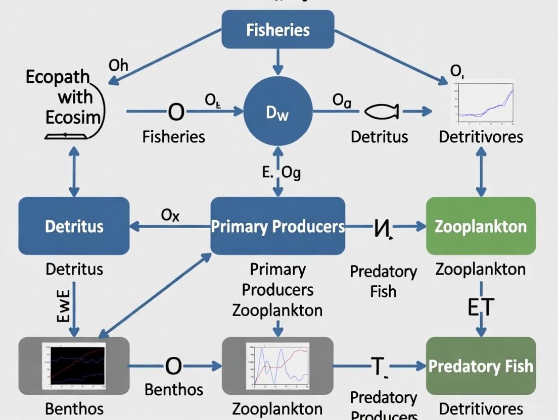
Diagram 1: EwE Modeling Workflow. This flowchart illustrates the sequential process of developing Ecopath, Ecosim, and Ecospace models, highlighting the foundational nature of Ecopath and the iterative relationships between dynamic simulation components.
Case Studies of Regional Applications
North Sea Historical Ecosystem Modeling
A pioneering application of EwE in the North Sea demonstrates the value of historical ecosystem reconstruction for establishing baseline conditions. Researchers developed two mass-balanced Ecopath models with identical topology to represent the North Sea ecosystem in the 1890s and 1990s, based on historical landings data from the 'Fishery Board for Scotland' [24].
The 1890s period represents the onset of industrial fisheries, while the 1990s was selected as a more recent reference point aligned with existing models used in current ecosystem-based management. This comparative approach revealed that direct and indirect impacts of fisheries on the food web triggered cascading changes in trophic interactions, ultimately leading to a decline in the ecosystem's maturity and resilience over the century [24]. The indicator-based assessment demonstrated that present-day model-based fisheries management practices in the North Sea rely on ecosystem structures that were already degraded, highlighting the importance of historical perspectives for setting appropriate restoration targets.
Table 2: Ecosystem Indicators for EwE Model Assessment and Comparison
| Indicator Category | Specific Metrics | Ecological Interpretation | Management Relevance |
|---|---|---|---|
| Trophic Structure | Mean Trophic Level of Catch, Trophic Pyramid Shape | Energy flow efficiency, ecosystem maturity | Sustainable harvesting patterns |
| Energy Flow | Total System Throughput, Finn's Cycling Index | Ecosystem productivity, nutrient recycling | Capacity to sustain fisheries |
| Ecosystem Organization | Ascendancy, Overhead | System development, resilience | Resistance to perturbations |
| Food Web Characteristics | Connectance, Omnivory Index | Trophic complexity, interaction diversity | Buffer against species loss |
| Fisheries Impact | Fishing Pressure, Primary Production Required | Ecosystem-level effects of fishing | Overall fisheries sustainability |
| Biomass Distribution | Total Biomass, Biomass of Top Predators | Ecosystem health, structural integrity | Conservation status |
Hawaiian Islands Coral Reef Ecosystem Management
Beyond European waters, EwE models have been successfully applied to coral reef ecosystems, demonstrating the approach's global relevance. In the Main Hawaiian Islands, researchers developed a social-ecological system (SES) conceptual framework to integrate human dimensions into EBFM [10] [25]. The model simulated four gear/species restrictions for the reef-based fishery, two fishing scenarios associated with the opening of hypothetical no-take Marine Protected Areas, and a Constant Effort (No Action) scenario [10].
This approach enabled quantification of trade-offs among societal objectives, supporting managers in choosing among alternative interventions. The model incorporated both ecological parameters (biomass, production rates, diet compositions) and social-economic parameters (fishery value, costs) to evaluate management scenarios in terms of their ability to improve ecosystem services that benefit human users [25]. The study demonstrated that when social and economic objectives are explicitly defined, EwE models can visualize and quantify management trade-offs, addressing a critical gap in conventional EBFM approaches.
Advanced Methodological Protocols
Best Practices for Model Development and Validation
As EwE applications have expanded, the community has established formal best practices to ensure model reliability and appropriate application:
- Uncertainty Analysis: Incorporate uncertainty assessment using the Ecosampler plug-in and Monte Carlo routines to evaluate parameter sensitivity and model robustness. Notably, only one-third of reviewed European publications incorporated comprehensive uncertainty analysis [21] [11].
- Ecological Network Analysis: Utilize Ecological Network Analysis (ENA) indices to summarize ecosystem structure and functioning. The ECOIND plug-in provides standardized calculation of ecological indicators for ecosystem state assessment [21].
- Model Balancing Techniques: Apply thermodynamic and ecological diagnostics to verify mass balance. This includes checking for realistic ecotrophic efficiency values (typically <1), appropriate production-to-consumption ratios, and credible biomass accumulation rates [11].
- Temporal Dynamic Fitting: Implement formal fitting procedures when calibrating Ecosim models to time series data, using statistical goodness-of-fit measures to evaluate model performance and identify potential ecosystem regime shifts [11].
- Spatial Explicit Modeling: Use Ecospace for spatiotemporal analysis, particularly when evaluating marine protected areas or habitat-specific management strategies. Ecospace allows representation of heterogeneous environments and species distributions [21] [23].
Integration with Management Frameworks
EwE models have proven particularly valuable in supporting regional and international management frameworks:
- EU Marine Strategy Framework Directive (MSFD): EwE models contribute to assessing Good Environmental Status (GEnS), particularly for biodiversity and food web descriptors. Models can demonstrate linkages between indicators and ecosystem structure/function, and evaluate impacts of pressures on ecosystem state [26].
- Common Fisheries Policy (CFP): EwE applications help implement the ecosystem approach to fisheries management required under the revised CFP, exploring multispecies interactions and trade-offs between conservation and exploitation objectives [21] [24].
- Ecosystem-Based Fisheries Management (EBFM): The models facilitate EBFM by quantifying trade-offs between ecological, economic, and social objectives, moving beyond single-species management to address ecosystem complexity [10].
Diagram 2: EwE Model Integration with Management Frameworks. This diagram shows how EwE models generate specific outputs that support different management frameworks and contribute to informed decision-making in marine resource management.
Table 3: Essential Research Tools for EwE Modeling Applications
| Tool/Resource | Type | Function | Access/Platform |
|---|---|---|---|
| EwE Software Suite | Modeling Software | Core platform for Ecopath, Ecosim, and Ecospace modeling | Free download from ecopath.org |
| EcoBase | Database Repository | Open-access repository of published EwE models for comparison and meta-analysis | Online database (ecobase.ecopath.org) |
| Ecosampler Plug-in | Uncertainty Module | Assess parameter uncertainty through Monte Carlo routines | Integrated in EwE software |
| ECOIND Plug-in | Indicator Tool | Quantitative calculation of standardized ecological indicators | Integrated in EwE software |
| Ecotracer Module | Contaminant Tracking | Model movement and accumulation of contaminants and radioisotopes | Integrated in EwE software |
| ENA Toolbox | Network Analysis | Ecological Network Analysis for evaluating ecosystem properties | Available within EwE suite |
| Time Series Data | Empirical Data | Fisheries catches, abundance indices, environmental variables | Region-specific datasets |
| Diet Composition Data | Biological Data | Quantitative predator-prey relationships | Literature review, stomach content analysis |
The global and regional applications of Ecopath with Ecosim models demonstrate their vital role in advancing ecosystem-based approaches to marine management. In European seas, the proliferation of EwE models has provided critical insights into ecosystem functioning, fisheries impacts, and potential management pathways under changing environmental conditions. The historical modeling approaches, such as those applied in the North Sea, offer valuable baselines for assessing ecosystem change and establishing restoration targets.
The continued development of EwE methodology, including improved uncertainty analysis, standardized ecological indicators, and more integrated social-ecological frameworks, strengthens its utility for addressing complex management challenges. As marine ecosystems face increasing pressures from climate change, fishing, and other human activities, the ability to simulate ecosystem dynamics and evaluate trade-offs among management objectives becomes increasingly essential for achieving sustainable ocean governance.
Building and Applying EwE Models: From Theory to Management Practice
Step-by-Step Guide to Constructing a Mass-Balanced Ecopath Model
Ecosystem-Based Fisheries Management (EBFM) is a holistic approach that integrates the dynamics of entire ecosystems, including societal dimensions, to achieve sustainable resource use [10]. The Ecopath with Ecosim (EwE) modeling framework serves as a cornerstone for implementing EBFM, providing a quantitative tool to visualize and quantify trade-offs among societal objectives and ecological constraints [10] [21]. Within this framework, constructing a mass-balanced Ecopath model is a critical first step, creating a static, mass-balanced snapshot of the ecosystem that serves as the foundation for temporal and spatial simulations [16] [21]. A mass-balanced model ensures that the energy flow within the ecosystem is mathematically plausible, meaning that for each functional group, energy consumption equals the sum of production, respiration, and unassimilated components [12]. This equilibrium state is essential for producing reliable simulations of management scenarios, climate change impacts, and other anthropogenic stressors [21].
Theoretical Foundation: The Master Equations of Ecopath
The Ecopath approach is built upon two master equations that govern the energy flow through each functional group in the model.
The First Master Equation: Energy Balance
The fundamental equation describing energy balance for each functional group is [12]:
Consumption = Production + Respiration + Unassimilated Part
This can be expressed mathematically as:
[ C = P + R + U ]
Where:
- ( C ) = Total consumption (biomass × consumption/biomass ratio)
- ( P ) = Total production (biomass × production/biomass ratio)
- ( R ) = Respiration (non-usable energy currency)
- ( U ) = Unassimilated part (egested or excreted portion of consumption)
For models with energy as currency, the unassimilated food default is typically 0.20 (20% of consumption) for finfish groups, though this can vary [12]. The unassimilated portion is directed to the detritus group.
The Second Master Equation: Production Allocation
The second master equation describes how production is utilized within the system [12] [18]:
Production = Predation Mortality + Fishing Mortality + Biomass Accumulation + Net Migration + Other Mortality
This can be expressed mathematically as:
[ P = M2 + F + BA + E + M0 ]
Where:
- ( P ) = Total production
- ( M2 ) = Predation mortality (consumption by predators)
- ( F ) = Fishing mortality (catch)
- ( BA ) = Biomass accumulation rate
- ( E ) = Net migration (emigration - immigration)
- ( M0 ) = Other mortality (diseases, senescence, etc.)
Table 1: Key Parameters for Ecopath Functional Groups
| Parameter | Symbol | Description | Unit | Typical Range |
|---|---|---|---|---|
| Biomass | B | Average biomass over the modeled period | t·km⁻² | Variable |
| Production/Biomass | P/B | Instantaneous mortality rate | year⁻¹ | 0.1-50 |
| Consumption/Biomass | Q/B | Consumption rate per unit biomass | year⁻¹ | 1-100+ |
| Ecotrophic Efficiency | EE | Proportion of production used in system | Unitless | 0-1 |
| Unassimilated Food | U | Proportion not assimilated | Unitless | 0.2 default |
Step-by-Step Protocol for Mass Balancing
Phase I: Data Collection and Parameter Estimation
Step 1: Define Functional Groups
- Identify and define the key species or functional groups representing the ecosystem structure
- Balance resolution (number of groups) with data availability and model objectives
- Recent models show increasing complexity over time, with some exceeding 50 functional groups [21]
Step 2: Collect Input Data For each functional group, compile the best available data for:
- Biomass (B) estimates from surveys or literature
- Production/Biomass (P/B) ratios from empirical relationships or literature
- Consumption/Biomass (Q/B) ratios from physiological models or literature
- Diet compositions from stomach content analysis or literature
- Fisheries catches (C) from official statistics or surveys
Step 3: Estimate Missing Parameters
- Ecopath can estimate one missing parameter per group (typically B, P/B, Q/B, or EE)
- The software uses a system of linear equations and matrix inversion to estimate missing values [12]
- Ensure diet compositions sum to 1 for each predator group [18]
Phase II: Initial Model Balancing
Step 4: Run Initial Parameter Estimation
- Execute the initial Ecopath parameter estimation routine
- The program will estimate missing parameters and provide initial balancing [18]
- Monitor for warning messages in the Status panel [18]
Step 5: Evaluate Initial Results Check the initial output for physiological and ecological plausibility:
- Ecotrophic Efficiency (EE): Must be between 0 and 1 [12]
- Gross Food Conversion Efficiency (g = P/Q): Typically 0.1-0.3 for most groups, lower for top predators, higher for small organisms [12]
- Respiration/Biomass (R/B) ratios: Should reflect activity levels (e.g., 1-10 year⁻¹ for fish, 50-100 year⁻¹ for copepods) [12]
Table 2: Troubleshooting Common Mass Balance Problems
| Problem | Possible Causes | Solution Approaches |
|---|---|---|
| EE > 1 | Overestimated predation, underestimated production | Adjust diet compositions, review P/B and Q/B values |
| Negative Respiration | P/Q + U/Q exceeds 1 | Lower P/B or increase Q/B, reduce unassimilated food proportion |
| Implausible g (P/Q) | Incorrect P/B or Q/B ratios | Compare with physiological expectations, consult literature |
| High R/B ratios | Underestimated production or overestimated consumption | Review basic input parameters, adjust unassimilated food |
Step 6: Apply the Fixed Selectivity Principle for Diet Composition For predators with generalized prey categories (e.g., "small fish"), use the fixed selectivity principle to distribute diet proportions based on prey productivity [12]:
[ DC{ji} = \frac{Bi \cdot (P/B)i}{\sum{k=1}^n Bk \cdot (P/B)k} ]
Where ( DC{ji} ) is the proportion of prey ( i ) in the diet of predator ( j ), ( Bi ) is the biomass of prey ( i ), and ( (P/B)_i ) is the production/biomass ratio of prey ( i ) [12].
Phase III: Iterative Refinement and Validation
Step 7: Analyze Mortality Rates
- Examine the Mortality Rates form (Ecopath > Output > Mortality rates > Mortalities) [18]
- Identify which mortality component (predation vs. fishing) is causing balancing issues [12]
- Use the Predation Mortality form to identify quantitatively important predators [12]
Step 8: Refine Parameters Iteratively
- Make incremental changes to parameters with highest uncertainty
- Document all changes and reasoning thoroughly [12]
- Save the data file under new names after significant changes [12]
Step 9: Evaluate Ecosystem Indicators
- Check system-level properties and indicators for plausibility
- Use network analysis plugins (ENA, ECOIND) for additional validation [21]
- Compare with similar ecosystems or previously published models
Table 3: Essential Tools and Resources for Ecopath Modeling
| Tool/Resource | Type | Function/Purpose | Availability |
|---|---|---|---|
| EwE Software | Modeling Platform | Core modeling environment with Ecopath, Ecosim, Ecospace modules | Free download [16] |
| EcoBase | Database | Repository of published EwE models for comparison | Open-access [21] |
| Ecosampler | Plug-in | Assess parameter uncertainty through Monte Carlo routine | Included in EwE [21] |
| ECOIND | Plug-in | Calculate standardized ecological indicators | Included in EwE [21] |
| Ecotracer | Plug-in | Model contaminants and radioisotopes in food webs | Included in EwE [21] |
| ENA Tool | Routine | Ecological Network Analysis for ecosystem indicators | Included in EwE [21] |
Workflow Visualization: Mass Balancing Procedure
Mass Balancing Workflow Diagram: This flowchart illustrates the iterative process of achieving mass balance in Ecopath models, highlighting key decision points and refinement procedures.
Advanced Applications in Fisheries Management Research
Mass-balanced Ecopath models serve as the foundation for dynamic simulations that address critical fisheries management questions. The balanced baseline model can be used to:
Evaluate Fishery Management Scenarios
- Test gear restrictions, catch limits, and spatial management measures [10]
- Quantify trade-offs between ecological, economic, and social objectives [10]
- Optimize policy decisions using EwE's policy optimization module [21]
Assess Environmental Impacts
- Model climate change effects on ecosystem structure and function [21]
- Evaluate impacts of alien species, pollution, and habitat modification [21]
- Analyze cumulative effects of multiple stressors [21]
Support Strategic Management Planning
- Implement Marine Protected Areas using Ecospace [16] [21]
- Track contaminants through food webs using Ecotracer [21]
- Model socioeconomic benefits using value chain modeling [21]
Constructing a mass-balanced Ecopath model requires both scientific rigor and practical problem-solving. Key best practices include:
- Documentation: Thoroughly document all parameter sources, assumptions, and changes made during balancing [12]
- Iterative Approach: Make small, justified changes and evaluate their effects systematically [12]
- Uncertainty Analysis: Use Ecosampler and Monte Carlo routines to incorporate parameter uncertainty [21]
- Peer Validation: Compare results with similar ecosystems and seek expert feedback
- Model Complexity: Balance resolution with data availability, acknowledging that "all models are wrong, but some are useful"
A properly mass-balanced Ecopath model provides not just a snapshot of ecosystem structure, but a powerful foundation for exploring dynamic management scenarios that support Ecosystem-Based Fisheries Management and the conservation of marine resources for future generations.
Ecopath with Ecosim (EwE) represents a pivotal methodology in ecosystem-based fisheries management, integrating a static, mass-balanced snapshot of an ecosystem (Ecopath) with dynamic simulation capabilities (Ecosim) [23]. The transition to temporal dynamics through Ecosim enables researchers to explore policy options, evaluate ecosystem effects of fishing, and analyze impacts of environmental changes [23]. This application note provides detailed protocols for configuring Ecosim for time-series simulations, framed within a broader thesis on advancing fisheries management research. The core of Ecosim's dynamic simulation lies in a system of differential equations that express biomass flux rates among pools as functions of time-varying biomass and harvest rates [27]. For researchers and scientists, mastering time-series configuration is essential for transforming static ecosystem snapshots into powerful predictive tools that can replicate historical patterns and explore future management scenarios.
Theoretical Foundation of Ecosim Dynamics
Ecosim utilizes a system of coupled differential equations to simulate biomass dynamics over time, building upon the initial mass-balanced conditions established in Ecopath [27] [28]. The fundamental equation governing biomass dynamics for each functional group (i) takes the form:
Figure 1. Conceptual structure of the core Ecosim differential equation for biomass dynamics [27].
Where dB_i/dt represents the growth rate of group (i) during time interval dt; g_i is the net growth efficiency; the summations represent consumption rates; Q_ij represents consumption by group i; Q_ji represents predation on group i; I_i is immigration rate; F_i is fishing mortality rate; e_i is emigration rate; and M0_i is the non-predation natural mortality rate [27]. The initial biomasses, rate parameters, and consumption flows are inherited from the base Ecopath model, creating a seamless transition from static to dynamic modeling.
Predator-prey interactions in Ecosim are moderated through foraging arena theory, which divides prey biomass into vulnerable and invulnerable components [27] [28]. The transfer rate (v_ij) between these components determines whether control is top-down (Lotka-Volterra type) or bottom-up (donor-driven) [27]. This theoretical framework allows Ecosim to simulate complex trophic cascades and ecosystem responses to fishing pressure and environmental changes.
Time Series Data Requirements and Structures
Time Series Classification and Specifications
Ecosim incorporates two primary categories of time series data: driver series that force the model (e.g., fishing effort) and reference series for fitting model predictions to observed data (e.g., biomass surveys) [29]. The software supports multiple data types, each with specific applications in fisheries research, as detailed in Table 1.
Table 1. Time series types available in Ecosim for model forcing and validation [30].
| Time Series Type | Unit | Abbreviation | Type Code | Pool Code | Pool Code 2 | Driver/Reference |
|---|---|---|---|---|---|---|
| Biomass, relative | – | BiomassRel | 0 | Group | – | Reference |
| Biomass, absolute | t·km⁻² | BiomassAbs | 1 | Group | – | Reference |
| Fishing effort | – | FishingEffort | 3 | Fleet | – | Driver |
| Fishing mortality | year⁻¹ | FishingMortality | 4 | Group | – | Driver |
| Total mortality | year⁻¹ | TotalMortality | 5 | Group | – | Reference |
| Catches | t·km⁻²·year⁻¹ | Catches | 6 | Group | – | Reference |
| Forcing function | – | TimeForcing | 2 | Function # | – | Driver |
| Landings, absolute | t·km⁻²·year⁻¹ | Landings | 12 | Fleet | Group | Reference |
Time Series File Configuration Protocol
Time series data must be structured in a specific comma-separated value (CSV) format for Ecosim compatibility. The configuration protocol consists of these critical steps:
- Header Configuration: The first row contains time series titles corresponding to functional groups or fleets in the model [29].
- Weight Assignment: The second row specifies weights for reference time series, representing prior assessment of data reliability (low weights indicate high variance or unreliable data) [31] [29].
- Pool Coding: The third row assigns numerical codes linking each time series to specific model components:
- Fleet numbers for effort data
- Functional group numbers for biomass and mortality data
- Forcing function numbers for environmental drivers [29]
- Type Specification: The fourth row identifies time series types using numerical codes or descriptive abbreviations (see Table 1) [29].
- Temporal Data Entry: Subsequent rows contain annual time series values, with driver series requiring complete annual entries to avoid null values [29].
Critical Implementation Note: Researchers must verify that group and fleet numbers in the CSV file correspond exactly to those in the Ecopath model, as discrepancies will cause integration failures [29].
Experimental Protocol: Time Series Fitting and Model Calibration
Preliminary Model Configuration
- Data Integration: Import the formatted CSV time series file via
Ecosim > Input > Time series[29]. - Baseline Simulation: Execute an initial Ecosim run (
Ecosim > Output > Run Ecosim > Run) without parameter optimization [29]. - Visual Diagnostics: Examine
Ecosim > Output > Ecosim group plotsto identify discrepancies between simulated trajectories and observed data [29].
Vulnerability Parameter Optimization
The vulnerability multiplier defines how predation mortality responds to changes in predator and prey abundance, representing how far a group is from its carrying capacity [29] [28]. The optimization protocol proceeds as follows:
- Parameter Initialization: Reset all vulnerability multipliers to default values (typically 2.0) via
Ecosim > Input > Vulnerabilities[29]. - Sensitivity Analysis:
- Navigate to
Ecosim > Tools > Fit to time series - Set
No of blocksto 1 - Select
By predatoroption - Execute
Sensitivity of SS to Vto identify parameters with greatest influence on model fit [29]
- Navigate to
- Iterative Parameter Search:
- Initiate search routine to optimize vulnerability parameters
- Progressively increase search complexity (blocks and parameters)
- Record Sum of Squared residuals (SS) and Akaike Information Criterion (AICc) values for model selection [29]
- Convergence Validation: Repeat optimization until additional parameters no longer significantly improve goodness-of-fit metrics [29].
Primary Production Anomaly Detection
Environmental variability can be incorporated through forcing functions that represent historical productivity regime shifts:
- Forcing Function Application: Apply pre-defined forcing functions to primary producer groups via
Ecosim > Input > Forcing function > Apply FF[29]. - Anomaly Search Configuration:
- Access
Ecosim > Tools > Fit to time series - Deactivate vulnerability search
- Activate anomaly search
- Reset all forcing functions via
Forcing function tab[29]
- Access
- Spline Point Optimization:
- Specify number of spline points (initially 2-3)
- Execute search routine
- Iteratively increase spline point complexity while monitoring AICc for overfitting [29]
- Integrated Optimization: Conduct combined vulnerability and anomaly searches for comprehensive model calibration [29].
Figure 2. Sequential workflow for Ecosim time series fitting and model calibration.
Goodness-of-Fit Evaluation and Model Diagnostics
Ecosim generates a statistical measure of goodness-of-fit calculated as a weighted sum of squared deviations (SS) of log biomasses from log predicted biomasses [31] [23]. For relative abundance data, this is scaled by the maximum likelihood estimate of the relative abundance scaling factor in the equation y = qB (where y = relative abundance, B = absolute abundance) [31]. Model selection should employ the Akaike Information Criterion (AICc) to balance fit quality against model complexity, preventing overfitting [29] [11].
The Scientist's Toolkit: Essential Research Reagents
Table 2. Essential computational tools and conceptual components for Ecosim time series analysis.
| Research Reagent | Function | Application Context |
|---|---|---|
| Vulnerability Multiplier | Modulates predator-prey interaction strength | Determining top-down vs. bottom-up control in trophic dynamics [29] |
| Forcing Function | Incorporates environmental drivers | Modeling temperature, productivity anomalies [29] [28] |
| Sum of Squares (SS) | Goodness-of-fit metric | Quantifying mismatch between observations and predictions [31] |
| Akaike Information Criterion (AICc) | Model selection criterion | Balancing fit quality and parameter complexity [29] [11] |
| Spline Points | Flexible curve fitting | Estimating annual primary production anomalies [29] |
| Pool Codes | Numerical identifiers | Linking time series data to model components [29] |
Applications in Ecosystem-Based Fisheries Management
The integration of time series data facilitates Ecosim's application to pressing fisheries management challenges. The calibrated dynamic models enable researchers to:
- Explore Fishing Policy Options: Test alternative fishing mortality scenarios and effort allocation strategies [23]
- Evaluate Ecosystem Effects: Analyze trophic cascades and unintended consequences of single-species management [31] [23]
- Assess Environmental Impacts: Quantify combined effects of fishing pressure and environmental change [31] [28]
- Optimize Management Strategies: Identify policies that balance ecological, economic, and social objectives [23]
Formal optimization approaches in Ecosim can maximize multi-objective functions incorporating fisheries profit, social benefits, species rebuilding mandates, and ecosystem structure [23]. This enables a rigorous, ecosystem-based approach to fisheries management that acknowledges the multifaceted nature of marine resource decision-making.
Configuring Ecosim for time-series simulations represents a critical transition from static ecosystem description to dynamic prediction in fisheries research. The protocols outlined in this application note provide researchers with a comprehensive framework for integrating time series data, calibrating model parameters, and validating dynamic ecosystem simulations. By adhering to these methodologies, scientists can enhance the predictive capacity of their ecosystem models, ultimately supporting more effective, evidence-based fisheries management decisions. The robustness of resulting management advice depends critically on proper time series configuration, parameter estimation, and model diagnostics—processes that transform Ecopath models from historical snapshots into powerful tools for exploring future ecosystem dynamics.
In the move toward Ecosystem-based Fisheries Management (EBFM), a critical scientific question is how different species or ecosystem components respond to various forcing factors and what the consequences are for management [32]. Forcing factors are external drivers that influence ecosystem dynamics; in marine contexts, the primary categories are top-down forcing (e.g., fishing pressure, which exerts control from higher trophic levels) and bottom-up forcing (e.g., primary production, which controls energy input from the base of the food web) [32]. Teasing apart the effects of these multiple, often confounding, factors is complex due to their potential for synergistic or antagonistic interactions [32].
Ecosystem models, particularly the Ecopath with Ecosim (EwE) software suite, are at the forefront of this research because ecosystem-scale experiments are rarely practicable [32]. The EwE approach provides a quantitative framework for investigating the relative influence of these drivers, allowing researchers to test hypotheses about their impacts and communicate these findings clearly to managers tasked with developing ecosystem management plans [32]. This document outlines the application and protocols for incorporating these forcing factors into EwE models, supporting advanced fisheries management research.
Key Forcing Factors in Marine Ecosystem Models
Categorization and Definitions
Marine ecosystem dynamics are influenced by a combination of anthropogenic and environmental drivers. The table below summarizes the primary forcing factors considered in EwE modelling.
Table 1: Key Forcing Factors in EwE Models
| Category | Specific Factor | Type of Forcing | Impact on Ecosystem |
|---|---|---|---|
| Anthropogenic | Fishing Mortality/Effort [32] | Top-down | Direct biomass removal, altering food-web structure and biodiversity [32]. |
| Marine Protected Areas [16] | Top-down | Spatial management altering mortality and fishing pressure. | |
| Chemical Pollution [21] | Bottom-up/Top-down | Can affect health of organisms and water quality. | |
| Infrastructure & Energy Production [21] | Habitat | Alters physical habitat and ecosystem structure. | |
| Environmental | Primary Production [32] | Bottom-up | Controls energy input, propagated through the food-web [32]. |
| Climate Change (e.g., Temperature) [21] | Bottom-up | Affects physiological rates, species distribution, and recruitment. | |
| Alien Species [21] | Top-down/Bottom-up | Introduces new competitors/predators, altering existing interactions. |
Relative Importance of Drivers
A comparative analysis of nine ecosystem models revealed that in all but one system (the North Sea), a combination of top-down forcing by fishing and bottom-up forcing of primary production yielded the best overall model representations of historical biomass trends [32]. Fishing effects were the stronger force in six of the nine systems, confirming its profound role in shaping exploited fish stocks [32]. However, in systems like the Irish Sea, East China Sea, and Southern Humboldt, the improvement from adding primary production forcing was more than double that from using fishing alone, indicating that bottom-up processes can be the dominant influence in some ecosystems [32].
Protocols for Incorporating Forcing Factors in EwE
General Workflow for Temporal Simulations (Ecosim)
The foundational protocol for investigating forcing factors in EwE involves using the Ecosim module for time-dynamic simulation. The general workflow for setting up and running these simulations is outlined below.
Diagram 1: General Ecosim workflow for forcing factor analysis.
Detailed Experimental Protocol:
Initial Ecopath Model: Begin with a mass-balanced static Ecopath model that provides a snapshot of the ecosystem for a base year [16] [10]. This model includes functional groups, their biomasses, production/consumption rates, and diet compositions.
Load Time Series Data: Import time series of observed data for fitting, which typically include:
Define Forcing Functions: Forcing functions are used to drive changes in the model externally.
- Fishing Forcing: Implemented by forcing fishing mortality rates or effort for specific fleets over time [32].
- Primary Production Forcing: Applied as a multiplier on the primary production (PP) rate of phytoplankton groups. The values for the first year should average 1 [33].
- Other Environmental Forcing: Can be applied to affect the productivity or consumption of specific functional groups [21].
Model Fitting and Calibration: Use Ecosim to fit the model to the loaded time series. This process involves adjusting parameters (e.g., vulnerabilities of prey to predators, which determine top-down vs. bottom-up control) to minimize the sum of squares (SS) between model predictions and observed data [32]. The Monte Carlo Ecosampler plug-in can be used to incorporate parameter uncertainty during this process [21].
Scenario Analysis: Once the model is satisfactorily fitted to past data, run future scenarios to explore policy options. Examples include:
Advanced Protocol: Multi-Scenario Analysis with the Multi-Sim Plug-in
For robust analysis, testing multiple forcing scenarios efficiently is crucial. The Multi-sim plug-in allows for multiple simulations, changing one or multiple forcing functions without uploading files individually [33].
Protocol for Multi-Sim:
Prepare CSV Input Files: Create one or more CSV files containing the forcing function data. Each file will trigger one simulation.
- The name of the forcing function in the CSV must match exactly the name of an existing forcing function in the EwE model [33].
- The file should contain only the data values, with no labels for time steps. If altering one forcing function, the CSV has one column; for multiple functions, it has multiple columns [33].
- The values for the first year must average 1 [33].
- The time steps (monthly or annual) must be consistent across all files and specified correctly in the plug-in.
Configure and Run Multi-Sim:
- Open your Ecosim scenario and ensure all base settings (mediations, effort) are correct.
- Navigate to
Ecosim > Tools > Multi-sim[33]. - Select Input Files: Use the "Choose" button to select all CSV files for your scenarios. You can select all files in a folder or individual files [33].
- Select Output Folder: Choose where to save results. Check "Create unique folder for every run" to avoid file overwriting [33].
- Choose Outputs: Select which result files (biomass, catch, etc.) to save for each simulation.
- Click "Run" to execute all scenarios.
Diagram 2: Multi-sim plug-in workflow for batch scenario processing.
Table 2: Essential Research Tools for EwE Forcing Factor Analysis
| Tool / Resource | Type | Function in Research | Relevant Link/Reference |
|---|---|---|---|
| Ecopath with Ecosim (EwE) | Core Software | Primary modeling environment for constructing Ecopath, Ecosim, and Ecospace models. | https://ecopath.org/ [16] |
| Multi-sim Plug-in | Software Plug-in | Enables batch execution of multiple simulations with different forcing function inputs. | EwE User Guide [33] |
| Ecosampler | Software Plug-in | Assesses parameter uncertainty by generating multiple model versions from probability distributions of input parameters. | [21] |
| ECOIND Plug-in | Software Plug-in | Calculates standardized ecological indicators from model output to assess ecosystem state and health. | [21] |
| EcoBase | Model Repository | An open-access database of published EwE models for meta-analysis and comparative studies. | http://ecobase.ecopath.org [21] |
| Time Series Data | Research Data | Historical data on biomass, catches, and environmental variables (e.g., from surveys, fisheries, satellites) for model fitting and forcing. | [32] [10] |
Application Case Study: Hawaiian Coral Reef Ecosystem
A practical application involved using EwE to support EBFM for the coral reef ecosystem of the Main Hawaiian Islands [10]. The objective was to better integrate human dimensions into evaluating fishery management scenarios.
- Model Setup: A social-ecological system (SES) framework was developed, leading to an Ecopath with Ecosim model. The model simulated ecological and social performance indicators [10].
- Forcing Factors and Scenarios: The study simulated several management interventions as forcing scenarios:
- Outcome: The approach demonstrated that by defining social, economic, and ecological objectives, EwE models can visualize and quantify trade-offs among societal objectives, providing a concrete tool for managers to choose among alternative interventions [10].
Incorporating forcing factors such as fisheries, primary production, and other environmental drivers is a cornerstone of applying the Ecopath with Ecosim approach to modern fisheries challenges. The protocols outlined—from basic Ecosim fitting to advanced multi-scenario analysis—provide a roadmap for researchers to systematically investigate the relative influence of these drivers. By leveraging these tools and methodologies, scientists can generate critical evidence to inform Ecosystem-based Fisheries Management, helping to navigate the complex trade-offs inherent in managing marine social-ecological systems.
Ecopath with Ecosim (EwE) is a premier ecosystem modeling software suite that has become an indispensable tool for fisheries scientists and marine ecologists. The suite comprises three core components: Ecopath for constructing static, mass-balanced snapshots of ecosystems; Ecosim for simulating temporal dynamics; and Ecospace, the spatial-temporal dynamic module designed for exploring impacts of marine protected areas (MPAs) and spatial management strategies [16]. This protocol focuses specifically on Ecospace, which enables researchers to simulate biomass distributions across seascapes, model trophic interactions in heterogeneous environments, and evaluate trade-offs between conservation and fisheries objectives through spatial management scenarios [2].
The integration of Ecospace within the broader EwE framework provides a powerful approach for implementing Ecosystem-Based Fisheries Management (EBFM). By translating Ecopath base models and Ecosim-calibrated dynamics into spatial dimensions, Ecospace allows investigators to address critical questions about habitat preferences, species distribution shifts, and the efficacy of MPAs under changing environmental conditions [2]. These capabilities are particularly valuable for supporting policies such as the European Union's Common Fisheries Policy (CFP) and Marine Strategy Framework Directive (MSFD), which require spatial planning tools that can balance ecological sustainability with socioeconomic considerations [34].
Theoretical Foundation of Ecospace
Core Algorithmic Principles
Ecospace operates on a raster-based framework that dynamically allocates biomass across a grid of spatial cells. The model incorporates habitat affinity indices for each functional group, which determine species distributions based on preferred environmental conditions and habitat types [2]. The spatial dynamics are driven by dispersal rates calculated from species mobility parameters, creating a simulation where biomass flows between adjacent cells according to concentration gradients.
The modeling framework incorporates trophic interaction rates that vary spatially based on the co-occurrence of predators and prey in each cell. This spatial explicit implementation of foraging arena theory represents a significant advancement over non-spatial models, as it allows for more realistic simulation of predator-prey interactions and bottom-up processes [2]. Additionally, fishing fleets with defined effort distributions interact with the spatial biomass, enabling analysts to evaluate fishery impacts under different management scenarios.
Integration with Ecopath and Ecosim
Ecospace derives its initial parameters from an Ecopath mass-balanced model, which provides the baseline biomass, production, consumption, and diet composition for each functional group. The time-dynamic parameters are then calibrated through Ecosim to match historical biomass and catch time series, ensuring that the spatial model reflects observed ecosystem dynamics [2]. This integrated approach maintains theoretical consistency across modeling scales while incorporating spatial heterogeneity that significantly influences ecosystem structure and function.
Table 1: Core Components of the Ecospace Modeling Framework
| Component | Description | Data Requirements |
|---|---|---|
| Base Map | Spatial grid defining the study area | Bathymetry, habitat classifications, geographic boundaries |
| Habitat Layers | Environmental parameters affecting species distribution | Temperature, salinity, primary production, seabed substrate types |
| Functional Group Parameters | Species- or group-specific habitat preferences | Habitat affinity indices, dispersal rates, foraging parameters |
| Fishing Fleet Definitions | Spatial distribution of fishing effort | Fleet-specific fishing grounds, gear characteristics, effort patterns |
| Management Scenarios | Configurations of MPAs and fishing restrictions | MPA boundaries, seasonal closures, gear restrictions |
Application Note: MPA Evaluation in the Aegean Sea
Study Design and Implementation
A recent implementation of Ecospace in the Aegean Sea demonstrates its application for evaluating MPA effectiveness amid ecological challenges including overexploitation and climate change [35]. Researchers developed a reference scenario projecting a 6% decline in total biomass by 2050, with more substantial decreases in commercially important species. This baseline established the context for evaluating five distinct management scenarios with varying MPA configurations and fishing restrictions.
The scenarios included: (1) fisheries prohibition within Natura 2000 areas; (2) extended protection within these designated zones; (3) expansion of bottom trawling and purse seining restrictions; (4) integration of offshore wind farms (OWFs) with associated fishing limitations; and (5) combinations of these spatial measures [35]. Each scenario was simulated through 2050, with outputs tracking biomass changes, spatial distribution shifts, and catch impacts for key functional groups.
Key Findings and Management Implications
Scenario analysis revealed that larger MPAs with stricter protections yielded more pronounced ecological benefits, particularly for demersal and benthic species. However, these conservation gains came with economic trade-offs, including reduced total catches in some cases [35]. Among the tested scenarios, Scenario 3 (extended bottom trawling and purse seining restrictions) demonstrated the highest biomass gains for key commercial species with moderate trade-offs in catch, making it particularly suitable for fisheries-focused management strategies.
The research also identified the potential for offshore wind farms to provide modest conservation benefits, suggesting opportunities for multi-use marine spatial planning [35]. The findings underscore the importance of context-specific scenario evaluation, as the performance of different MPA configurations varied significantly across species groups and spatial scales.
Table 2: Summary of Ecospace Scenario Results from Aegean Sea Case Study
| Scenario | Total Biomass Change | Commercial Species Biomass | Catch Impacts | Recommended Application |
|---|---|---|---|---|
| Reference | -6% decline by 2050 | Substantial decreases | Baseline | Business-as-usual projection |
| Scenario 1 | Localized increases | Moderate improvement | Variable reductions | Biodiversity conservation focus |
| Scenario 2 | Localized increases | Moderate improvement | Variable reductions | Enhanced conservation strategy |
| Scenario 3 | Significant localized gains | Highest improvement | Moderate trade-offs | Fisheries management focus |
| OWF Integration | Modest increases | Slight improvement | Minimal disruption | Multi-use spatial planning |
Experimental Protocols
Protocol 1: Ecospace Model Initialization
Objective: To construct a spatially explicit ecosystem model from an existing Ecopath and Ecosim foundation.
Materials and Software:
- Ecopath with Ecosim software version 6.6+ [16]
- Georeferenced base map of study area (shapefile or raster)
- Habitat classification layers (seabed substrates, depth zones)
- Environmental data layers (temperature, primary production)
Procedure:
- Load Base Model: Import the calibrated Ecopath/Ecosim model (.ewemdb file)
- Define Spatial Grid:
- Set grid cell resolution (typically 1-5 km depending on ecosystem extent)
- Define projection system appropriate for the study region
- Import Habitat Map:
- Load benthic broad habitat types (BBHTs) classification [34]
- Assign habitat productivity parameters for each functional group
- Configure Functional Groups:
- Set habitat affinity indices for each group across habitat types
- Define dispersal parameters based on species mobility
- Initialize Fishing Fleets:
- Map historical fishing effort distributions
- Assign gear-specific habitat access restrictions
Validation Steps:
- Verify mass balance is maintained in initial spatial distribution
- Check that model stabilizes under baseline conditions
- Confirm spatial patterns align with empirical distribution data
Protocol 2: MPA Scenario Implementation
Objective: To design and implement marine protected area scenarios for evaluating conservation and fisheries outcomes.
Materials:
- Initialized Ecospace model
- MPA boundary proposals (shapefiles)
- Fishing effort redistribution assumptions
Procedure:
- Scenario Definition:
- Delineate MPA boundaries using polygon import tools
- Specify protection levels (no-take, gear-specific restrictions)
- Define temporal aspects (permanent, seasonal closures)
- Fleet Response Configuration:
- Set effort redistribution rules (distance-based, habitat-based)
- Define economic adaptability parameters
- Simulation Parameters:
- Set run duration (typically 20-50 years for MPA evaluation)
- Configure output intervals for time series data
- Enable spatial indicator calculations
- Model Execution:
- Run baseline scenario without MPAs
- Execute each MPA scenario independently
- Implement replication runs for uncertainty assessment
Output Analysis:
- Extract biomass trajectories by functional group and region
- Calculate spatial indicators (biomass centroids, aggregation indices)
- Compare catch and value metrics across scenarios
- Generate trade-off analysis between conservation and fisheries objectives
Protocol 3: Climate Change Integration
Objective: To incorporate environmental drivers and climate change projections into Ecospace simulations.
Materials:
- Downscaled climate projections (temperature, pH, etc.)
- Species-specific environmental response functions
- Primary production anomalies from biogeochemical models
Procedure:
- Environmental Layer Preparation:
- Import time-series of environmental variables
- Convert to Ecospace-compatible format (ASCII grid or NetCDF)
- Response Function Definition:
- Assign temperature tolerance ranges for each functional group
- Set primary production forcing relationships
- Configure phenology shifts for seasonal species
- Coupled Model Execution:
- Run reference scenario with constant environmental conditions
- Execute climate scenarios with dynamic environmental forcing
- Compare outputs to isolate climate effects
Validation Metrics:
- Match historical distribution shifts where data exists
- Verify physiological responses align with experimental studies
- Confirm model stability under extreme environmental values
Visualization and Workflow
Figure 1: Ecospace Model Development Workflow. The diagram illustrates the sequential integration of Ecopath, Ecosim, and spatial data leading to scenario analysis.
The Scientist's Toolkit: Essential Research Reagents
Table 3: Essential Modeling Components for Ecospace Implementation
| Component | Specifications | Application in Research |
|---|---|---|
| EwE Software Suite | Version 6.6+ [16] | Core modeling platform with Ecospace capability |
| Benthic Broad Habitat Types (BBHTs) | High-resolution seabed substrate classification [34] | Defines habitat preferences and species distributions |
| Primary Production Forcing | Satellite-derived chlorophyll and productivity data [2] | Drives bottom-up processes in the ecosystem model |
| Fishing Effort Distribution | Vessel monitoring system (VMS) and logbook data | Spatial allocation of fishery impacts |
| Environmental Driver Data | Temperature, salinity, oxygen concentration [2] | Climate change scenario implementation |
| Habitat Affinity Indices | Species-specific habitat preference parameters [2] | Determines spatial distribution of functional groups |
Advanced Applications and Future Directions
The ongoing development of Ecospace within international research projects like EcoScope and MARHAB continues to expand its capabilities [2] [34]. Current innovations focus on integrating high-resolution spatial data from advanced seabed mapping technologies, incorporating socioeconomic analyses to evaluate livelihood impacts, and implementing uncertainty quantification frameworks such as Robust Decision Making (RDM) [2].
The RDM approach is particularly valuable for addressing deep uncertainty in future climate projections and socioeconomic drivers. Rather than seeking consensus on precise future conditions, RDM identifies management strategies that perform adequately across a wide range of plausible scenarios [2]. This approach is being implemented in European projects to evaluate fisheries management strategies under uncertain climate futures, strengthening the utility of Ecospace for adaptive management.
Future developments will further enhance the spatial resolution of models, improve the representation of human dimension processes, and strengthen linkages with biogeochemical models. These advances will position Ecospace as an increasingly vital tool for navigating the complex trade-offs between conservation objectives and sustainable resource use in rapidly changing marine ecosystems.
Defining and Achieving Ecosystem Reference Points for Fisheries Management
Ecological Reference Points (ERPs) are benchmarks used in fisheries management to compare the current status of a fishery system against a desirable state, while accounting for ecological and environmental processes that affect fish stock productivity [36]. The development of ERPs represents a pivotal shift from traditional single-species management approaches toward Ecosystem-Based Fisheries Management (EBFM), which considers species within their broader ecological context, particularly for forage fish that play critical roles in marine food webs [37] [38].
The fundamental principle behind ERPs is the recognition that fish stocks do not exist in isolation but are embedded within complex trophic networks where harvesting one species can have cascading effects on dependent predators and overall ecosystem structure [37]. This is especially relevant for forage species like Atlantic menhaden (Brevoortia tyrannus), which support both valuable commercial fisheries and serve as essential prey for numerous predatory species including striped bass, bluefish, and marine mammals [37]. The ERP approach quantitatively links the management of forage species to the conservation objectives of their predators, creating a framework for multispecies management that acknowledges ecological interdependencies [36].
Conceptual Framework of Reference Points
Types of Reference Points
Fisheries management employs several categories of reference points, each serving distinct functions in management systems [39] [40]:
- Target Reference Points (TRPs): Define the desirable fishery state that should be achieved and maintained. TRPs create a buffer zone to ensure that limit reference points are not breached and can be based on biological, ecological, social, or economic considerations.
- Limit Reference Points (LRPs): Define an undesirable biological state of the stock that should be avoided. To keep the stock safe, the probability of violating an LRP should be very low. If an LRP is violated, immediate management action is required to return the stock to the target level.
- Trigger/Threshold Reference Points: Benchmarks that activate pre-defined management responses to help the fishery remain close to the target reference point and avoid breaching the limit reference point, typically set between the TRP and LRP.
These reference points can be further categorized as either fishing mortality-based (F-based) or biomass-based (B-based). F-based reference points manage the rate of fishing mortality and can be directly controlled through management measures, while B-based reference points focus on maintaining stock biomass levels from an ecological perspective, which cannot be directly managed but are more intuitive for stakeholders [39].
Table 1: Categories of Fisheries Management Reference Points
| Reference Point Type | Management Function | Key Characteristics |
|---|---|---|
| Target (TRP) | Defines desirable fishery state | Creates buffer zone; based on multiple objectives |
| Limit (LRP) | Identifies undesirable state | Requires immediate action if breached; precautionary |
| Trigger/Threshold | Activates management response | Early warning system; between TRP and LRP |
| F-Based | Controls fishing mortality rate | Directly manageable; less intuitive |
| B-Based | Maintains biomass levels | Ecologically focused; more stakeholder-friendly |
ERP Conceptual Diagram
The following diagram illustrates the conceptual relationship between traditional single-species reference points and ecological reference points that account for predator-prey dynamics:
Methodology for ERP Development Using Ecopath with Ecosim
Ecopath with Ecosim Framework
Ecopath with Ecosim (EwE) is a trophic dynamic modeling package that facilitates management of biomass and food web data for whole ecosystems and has been widely used for analysis of aquatic resources [37]. The EwE framework consists of several integrated components:
- Ecopath: Provides a static, mass-balance snapshot of the ecosystem that accounts for trophic interactions among organisms at multiple trophic levels by describing matter and energy flows. It represents the production of each modeled species or functional group as allocated among fishing, predation, other mortality, and migration while maintaining mass-balance between groups [41] [37].
- Ecosim: Enables dynamic simulations using the mass-balanced model from Ecopath to project changes due to human activities (including fishing), climate change, and other time-varying processes. Ecosim models biomass dynamics through differential equations where the change in biomass for each group is predicted as its consumption minus losses to predation, fishing, and migration [41] [37].
- Ecospace: Provides a spatial component to the modeling framework, allowing simulation of the effects of different management options, such as controls on fishing effort and spatial closures, on both fished species and trophic interactions [41].
Models of Intermediate Complexity (MICE)
For ERP development, Models of Intermediate Complexity for Ecosystems (MICE) have emerged as particularly valuable tools [37]. MICE models strike a balance between overly simplistic single-species models that ignore key ecosystem interactions and highly complex end-to-end ecosystem models that have substantial data requirements and parameter uncertainty. These models include only the necessary components to address specific management questions, making them more accessible for management timelines while retaining critical ecological relationships [37].
The Northwest Atlantic Continental Shelf MICE (NWACS-MICE) model developed for Atlantic menhaden management reduced ecosystem complexity from 61-80 functional groups in the full ecosystem model to just 15-17 species/functional groups, focusing specifically on menhaden and their key managed predators [42] [37]. This simplification maintained the necessary resolution to evaluate tradeoffs in harvest policies while remaining computationally efficient enough for management applications.
Step-by-Step ERP Development Protocol
The development of ERPs using EwE follows a systematic five-step protocol:
Step 1: Ecosystem Model Development and Calibration
- Define functional groups based on ecological role and management significance
- Parameterize biological characteristics (biomass, production/consumption rates, diet composition)
- Calibrate the model to historical data to estimate predator-prey interaction parameters
- Validate model performance against independent data sources
Step 2: Estimate Single-Species Reference Points
- Conduct equilibrium projections for each managed species independently
- Establish traditional single-species target and threshold reference points (e.g., Ftarget and Fthreshold)
- Determine biomass targets and thresholds corresponding to these fishing mortality rates
Step 3: Equilibrium Projections with Multiple Stressors
- Run equilibrium projections under combinations of predator and prey fishing mortality rates
- Maintain other modeled species at status quo fishing levels
- Systematically explore the tradeoff space between prey harvest and predator biomass
Step 4: Analyze Tradeoff Relationships
- Plot predator biomass as a function of both predator and prey fishing mortality rates
- Identify contours where predator biomass equals management targets
- Quantify the sensitivity of different predators to changes in prey availability
Step 5: Establish Ecological Reference Points
- Identify the prey fishing mortality rates that maintain key predators at their biomass targets
- Designate these as ERP Ftarget and ERP Fthreshold for management
- Feed ERPs back into stock assessment models to provide information on total allowable catch
The following workflow diagram illustrates this ERP development process:
Case Study: Atlantic Menhaden ERP Development
Application to Atlantic Menhaden Management
Atlantic menhaden represent an ideal case study for ERP implementation, as they support the largest commercial fishery by weight on the U.S. East Coast while simultaneously serving as critical forage for numerous predator species [37]. The Atlantic States Marine Fisheries Commission (ASMFC) identified key management objectives for menhaden that included: (1) sustaining menhaden to provide for directed fisheries, (2) sustaining menhaden for consumptive needs of predators, (3) sustaining menhaden to provide stability across all fisheries, and (4) minimizing risk due to a changing environment [37].
The NWACS-MICE model identified striped bass (Morone saxatilis) as the predator most sensitive to menhaden harvest, leading to its selection as the primary indicator species for ERP development [37]. The ERPs were specifically defined as the menhaden fishing mortality rates that maintain striped bass at their biomass target and threshold when striped bass are fished at their Ftarget, with all other modeled species fished at status quo levels [37].
Quantitative ERP Results for Atlantic Menhaden
The ERP analysis yielded specific fishing mortality reference points for Atlantic menhaden management:
Table 2: Comparison of Single-Species and Ecological Reference Points for Atlantic Menhaden
| Reference Point Type | Fishing Mortality Rate | Relationship to Single-Species | Management Implications |
|---|---|---|---|
| Single-Species Ftarget | Not specified | Baseline | Traditional management approach |
| ERP Ftarget | 0.19 | 30-40% lower than single-species | Maintains striped bass at target biomass |
| ERP Fthreshold | 0.57 | 30-40% lower than single-species | Maintains striped bass at threshold biomass |
| 2017 Fishing Mortality | Lower than 0.19 | More conservative than ERPs | Existing management already precautionary |
These ERPs were formally adopted by the ASMFC Menhaden Management Board in 2020, marking the first implementation of inter-dependent multispecies reference points for a fishery system in the United States [36]. The adoption demonstrates how ecosystem modeling can directly inform management decisions and facilitate the transition to EBFM.
Research Toolkit: Essential Components for ERP Development
Successful development of ERPs requires specific methodological components and research tools. The following table outlines key elements necessary for implementing the EwE approach to ERP development:
Table 3: Research Toolkit for ERP Development Using Ecopath with Ecosim
| Research Component | Function in ERP Development | Data Requirements |
|---|---|---|
| Ecopath with Ecosim Software | Core modeling platform for ecosystem simulations | Open-source software with specialized modules for dynamics and spatial analysis |
| Functional Group Classification | Organizes species into ecologically similar units | Life history traits, feeding ecology, habitat use data |
| Diet Composition Matrix | Quantifies energy flows between functional groups | Stomach content analysis, stable isotope studies, literature reviews |
| Fishery Catch Time Series | Calibrates model to historical fishing patterns | Commercial and recreational landings, discards, fishing effort data |
| Biomass and Abundance Indices | Provides baseline and time-series for calibration | Fisheries-independent surveys, stock assessment results, hydroacoustic data |
| Parameter Estimation Algorithms | Estimates uncertain parameters through model fitting | Optimization routines, Monte Carlo sampling, statistical priors |
The development of Ecological Reference Points using Ecopath with Ecosim represents a significant advancement in fisheries management, moving beyond single-species approaches to address the complex trophic interactions that characterize marine ecosystems. The Atlantic menhaden case study demonstrates that ERPs can be practically implemented within existing management frameworks, providing a scientifically defensible method to balance fishery yields with ecosystem conservation objectives [37] [36].
Future directions in ERP research include incorporating spatial and seasonal dynamics to address localized depletion concerns, expanding model frameworks to include environmental drivers and climate change impacts, and developing ERPs for additional forage species and ecosystems [36]. The continued refinement of MICE models promises to make ecosystem-based management increasingly accessible for diverse fisheries, supporting the sustainable management of marine resources in a changing world.
Calibration and Optimization: Best Practices for Robust EwE Models
The Critical Role of Vulnerability Settings in Predator-Prey Interactions
In the Ecopath with Ecosim (EwE) modeling framework, vulnerability multipliers are crucial parameters that govern the dynamics of predator-prey interactions. These parameters (denoted as K or v) determine how predation mortality rates change in response to variations in predator and prey abundances, thereby influencing whether the ecosystem control is top-down (predator-driven) or bottom-up (prey-driven) [43].
The Ecosim module uses a foraging arena theory to simulate these interactions. In this concept, the prey biomass is dynamically divided into vulnerable and invulnerable components, with the vulnerability multiplier setting the maximum potential increase in predation mortality rate relative to the baseline Ecopath level [43]. Proper configuration of these parameters is essential for creating realistic simulations that can accurately inform Ecosystem-based Fisheries Management (EBFM).
Theoretical Foundation and Mathematical Formulation
Foraging Arena Theory
Ecosim implements the foraging arena concept through a system of differential equations where prey species (i) exist in two states: vulnerable (V~i~) and invulnerable (B~i~ - V~i~) to predation by predator j [43]. The flow between these states is controlled by an exchange rate v~ij~, which represents the behavioral or physical mechanisms that limit predation risk.
The vulnerable biomass available to predators is calculated as: V~ij~ = v~ij~B~i~ / (2v~ij~ + a~ij~P~j~) where a~ij~ is the predator rate of effective search, B~i~ is prey biomass, and P~j~ is predator biomass [43].
Linking Vulnerability Multipliers to Exchange Rates
The critical connection for model parameterization is that vulnerability exchange rates (v~ij~) are derived from vulnerability multipliers (k~ij~) using the Ecopath baseline predation mortality rate (M2~ij~): v~ij~ = k~ij~M2~ij~ [43]
The predator rate of effective search (a~ij~) is subsequently estimated as: a~ij~ = 2v~ij~ / [(k~ij~ - 1)P~0~] [44]
Table 1: Key Parameters in Ecosim Vulnerability Formulation
| Parameter | Symbol | Description | Typical Range |
|---|---|---|---|
| Vulnerability Multiplier | k~ij~ | Maximum relative increase in predation mortality | 1 to ∞ (default=2) |
| Vulnerability Exchange Rate | v~ij~ | Rate of movement between vulnerable/invulnerable states | Function of k~ij~ and M2~ij~ |
| Effective Search Rate | a~ij~ | Predator efficiency in finding prey | Derived from k~ij~ and P~0~ |
| Baseline Predation Mortality | M2~ij~ | Ecopath baseline predation mortality | From mass-balance |
Ecological Interpretation of Multiplier Values
The value of vulnerability multipliers determines the nature of control in predator-prey relationships:
- Low multipliers (near 1.0): Represent bottom-up control where predators are at their carrying capacity and cannot significantly increase predation pressure. Consumption increases are tied to prey productivity [43].
- High multipliers (>> 2.0): Represent top-down control where predators can substantially increase predation mortality rates, potentially causing trophic cascades [43].
- Default value (2.0): Assumes predation mortality can at most double from Ecopath baseline levels [43].
Practical Application and Configuration Protocols
Estimating Multipliers for Population Recovery
For predicting predator recovery under reduced fishing pressure, a minimum vulnerability multiplier can be estimated using: K = (R - 1)HP~0~ / (Q~0~/B~0~* - HP~0~) [44] where R is the target recovery ratio (P~unfished~/P~0~), *H = Z/(eB~0~), Z is natural mortality rate, and e is food conversion efficiency [44].
This approach assumes no prey depletion as the predator recovers, making it a minimum estimate that may need adjustment if key prey populations become limited [44].
Configuration Workflows for Different Scenarios
Figure 1: Workflow for configuring vulnerability settings in EwE applications, highlighting data-rich and data-limited pathways.
Multi-Stanza Population Considerations
For age-structured populations (multi-stanza groups), a more iterative approach is required [44]:
- Initial step: Set high K values for older stanzas to allow biomass-per-recruit increases
- Subsequent adjustment: If biomass response is insufficient, increase K for juvenile stanzas to enable both increased recruitment and maintained growth rates
- Balance: Calibrate to represent realistic density-dependent mortality and stock-recruitment relationships
Table 2: Vulnerability Configuration Approaches with Advantages and Limitations
| Approach | Methodology | Best For | Limitations |
|---|---|---|---|
| Statistical Fitting | Automated estimation using time series data and goodness-of-fit measures [23] [45] | Data-rich systems with extensive time series | May produce ecologically unrealistic values without careful validation [43] |
| A Priori Ecological Knowledge | Setting values based on known predator-prey dynamics and behavioral observations [43] | Data-poor systems or well-studied species | Subjective and dependent on expert availability |
| Trophic-Level Based (vTL) | Setting values correlated with trophic position [45] | Initial parameterization and exploratory models | May oversimplify complex interactions |
| Depletion-Based (vB) | Linking to stock depletion status [45] | Systems with known fishing history | Requires historical abundance information |
Research Reagent Solutions: Essential Modeling Components
Table 3: Essential Components for EwE Vulnerability Analysis
| Component | Function | Application in Vulnerability Setting |
|---|---|---|
| Time Series Data | Relative/absolute abundance, catch, fishing mortality, effort data [23] | Statistical estimation and validation of vulnerability multipliers through model fitting |
| Goodness-of-Fit Metrics | Sum of squares (SS) of deviations between predicted and observed values [23] | Sensitivity analysis and optimization of vulnerability parameters |
| Vulnerability Multiplier Interface | Ecosim > Input > Vulnerabilities > Estimate vulnerabilities [44] | Initial estimation of average prey vulnerability needed for predator recovery |
| Sensitivity Analysis Tools | Measurement of SS change with 1% vulnerability parameter changes [23] | Identification of parameters most critical for time series fits |
| Ecopath Baseline Parameters | Biomass, production/biomass, consumption/biomass, diet composition [23] | Foundation for calculating baseline predation mortality (M2) |
Experimental Protocols for Vulnerability Parameterization
Protocol 1: Statistical Fitting with Time Series Data
Purpose: To estimate vulnerability multipliers that minimize differences between simulated and observed time series data [23] [45].
Procedure:
- Compile time series data including relative abundance indices, absolute abundance estimates, catch, fishing effort, and mortality rates [23]
- Load reference data into Ecosim covering an appropriate historical period
- Run initial simulation with default vulnerability settings (k~ij~ = 2.0)
- Calculate goodness-of-fit measure as weighted sum of squared deviations (SS) of log biomasses [23]
- Perform sensitivity analysis by changing each vulnerability parameter slightly (1%) and measuring SS change [23]
- Execute optimization routine to search for vulnerability estimates that improve fit to time series data
- Block similar vulnerabilities into ecologically meaningful sets to reduce parameter dimensionality [23]
- Validate fitted parameters through ecological sense-checking and cross-validation [43]
Protocol 2: Data-Limited Parameterization
Purpose: To establish reasonable vulnerability settings when time series data are insufficient for statistical fitting [43].
Procedure:
- Categorize predator-prey relationships based on ecological knowledge (e.g., schooling behavior, habitat use, diel patterns)
- Apply trophic-level guidelines: Higher multipliers for upper trophic level predators [45]
- Incorporate depletion status: Adjust multipliers for exploited species based on historical fishing impacts [45]
- Use the recovery estimator for key predators: Ecosim > Input > Vulnerabilities > Estimate vulnerabilities [44]
- Set multi-stanza parameters: Lower values for juvenile stanzas to represent density dependence [44]
- Document ecological rationale for each major vulnerability decision
Protocol 3: Model Skill Assessment
Purpose: To evaluate hindcast and forecast performance of different vulnerability configurations [45].
Procedure:
- Configure multiple model versions with different vulnerability settings (fitted, vTL, vB, default)
- Reserve portion of time series for validation (hindcast skill assessment)
- Run simulations over historical period with known fishing patterns
- Calculate skill metrics: bias, error, and reliability measures [45]
- Compare observed vs. predicted biomass trajectories for key functional groups
- Test forecast skill under alternative management scenarios (e.g., reduced/increased fishing effort) [45]
- Select optimal configuration based on comprehensive skill assessment
Implications for Ecosystem-Based Fisheries Management
Proper vulnerability setting significantly affects EBFM policy evaluations in EwE:
- Fishery Recovery Predictions: Higher vulnerability multipliers allow more rapid predator recovery under reduced fishing but increase sensitivity to prey depletion [44] [43]
- Management Strategy Evaluation: Vulnerability-fitted models demonstrate superior hindcast abilities, supporting more reliable policy exploration [45]
- Uncertainty Characterization: Comparing multiple vulnerability settings (e.g., v-fitted, vTL, vB) provides bounds on prediction uncertainty [45]
- Tradeoff Analysis: Different vulnerability configurations can be tested against multiple policy objectives (rent maximization, social benefits, mandated rebuilding) [23]
Figure 2: Relationship between vulnerability settings, ecosystem control type, and management implications in EwE-based policy evaluations.
Within the context of fisheries management research using Ecopath with Ecosim (EwE), accurately calibrating ecosystem models to historical data is a critical step for producing credible policy simulations. A central challenge in this calibration process involves representing the consumption dynamics between predators and their prey. This application note details the experimental protocols and outcomes for comparing two distinct parameterization approaches for these dynamics: the predator vulnerability multiplier (kj) and the predator-prey vulnerability multiplier (kij). The predator multiplier applies a single, generalized vulnerability value for all prey of a given predator, simplifying model structure. In contrast, the predator-prey multiplier allows for unique, interaction-specific vulnerability values, offering greater detail but requiring more data for estimation. This research, framed within a broader thesis on EwE, systematically evaluates how these approaches emerge during model fitting, their sensitivity to data quality, and their subsequent impact on key fisheries management benchmarks.
Background and Definitions
In Ecosim, vulnerability multipliers determine how a prey group's biomass availability changes in response to predator abundance, shaping the functional response of predators. These multipliers control the flow of energy between trophic levels and thus fundamentally influence simulated population dynamics.
- Predator Vulnerability Multiplier (kj): This is a predator-specific parameter. A single
kjvalue is applied to all prey items in a given predator's diet, representing an average foraging efficiency or habitat overlap for that predator. It simplifies the model by reducing the number of parameters. - Predator-Prey Vulnerability Multiplier (kij): This is an interaction-specific parameter. A unique
kijvalue is defined for each distinct predator-prey link in the food web. This allows the model to represent highly specific ecological relationships, such as a prey species' particular defense mechanisms against a specific predator.
The choice between these approaches involves a trade-off between model complexity, parameter identifiability, and ecological realism. The kj approach is more parsimonious, while the kij approach can capture more nuanced ecosystem dynamics but is more susceptible to overfitting, especially with limited data.
Experimental Protocol: A Comparative Case Study
The following protocol, adapted from a formal case study on the Anchovy Bay ecosystem model, outlines a rigorous methodology for comparing the kj and kij fitting approaches [46].
Phase 1: Base Model and "True" Data Generation
Objective: To establish a controlled baseline by generating synthetic but ecologically plausible time series data.
- Define Fishing Effort Trends: Configure the EwE model with realistic, time-varying fishing effort for different fleets (e.g., exponential decline for sealers and trawlers, linear increase for seiners) [46].
- Set "True" Vulnerability Parameters:
- For the
kjscenario, assign a mix of high, low, and defaultkjvalues to key functional groups (e.g., seals, cod, whiting). For overexploited groups, use the "Estimate Vulnerabilities" interface to set values [46]. - For the
kijscenario, use the Ecosim sensitivity search to identify the ten most sensitive predator-prey interactions. Manually adjust thesekijparameters to ensure a range of high and low values [46].
- For the
- Generate "True" Time Series: Run Ecosim simulations using the configured effort and vulnerability parameters. Export the resulting biomass and catch trajectories for key functional groups. These are treated as error-free "real observations" [46].
- Introduce Data Noise: To simulate real-world observation error, create multiple calibration datasets by adding random, normally distributed noise to the "true" biomass trends. Prepare scenarios with Coefficients of Variation (CV) of 0 (no noise), 0.1, 0.3, and 0.5 [46].
Phase 2: Model Fitting and Parameter Re-emergence
Objective: To test whether the original "true" vulnerability parameters can be recovered through a standard fitting procedure under different data quality conditions.
- Reset Model Parameters: Reset all vulnerability multipliers in the model to the EwE default value of 2. Retain the original fishing effort time series [46].
- Stepwise Fitting Procedure: Use the manual, stepwise fitting interface in EwE. This iterative process involves [47]:
- Running the model and comparing outputs to the calibration time series.
- Identifying functional groups with large discrepancies between simulated and observed biomass trends.
- Focusing on high-biomass, ecologically important groups first.
- For each problematic group, systematically testing hypotheses (e.g., bad trend data, incorrect fishing mortality, inappropriate vulnerability settings) and adjusting parameters to improve fit.
- Execute Fitting Trials:
kjFitting: Using the calibration data (across all CV levels), estimate the predator vulnerability multiplierskjfor seals, cod, whiting, shrimp, benthos, and zooplankton [46].kijFitting: Using the same calibration data, estimate the predator-prey vulnerability multiplierskijfor the ten most sensitive predator-prey pairs identified earlier [46].
- Documentation: Meticulously document all emerging parameter values and the resulting model fits for each scenario. Recording alternative hypotheses and parameter changes during this process is critical for future analysis and research prioritization [47].
Phase 3: Impact Assessment on Management Metrics
Objective: To quantify how the differing vulnerability parameters obtained from each approach affect key fisheries management indicators.
- Simulate Carrying Capacity: For each fitted model, run a long-term simulation in the absence of fishing. Record the resulting carrying capacity for each functional group [46].
- Estimate FMSY: For each fitted model, use Ecosim's policy exploration tools to estimate the fishing mortality rate consistent with achieving Maximum Sustainable Yield (FMSY) for key commercial species [46].
- Compare to Baseline: Compare the carrying capacities and FMSY estimates from the fitted models (
kjandkij) against the values derived from the original "true" parameter model.
Table 1: Summary of Comparative Experimental Protocol
| Phase | Key Activity | Key Inputs | Key Outputs |
|---|---|---|---|
| 1. Base Model Setup | Generate "true" data | Pre-defined fishing effort; "True" kj or kij values | Synthetic biomass and catch time series (with/without noise) |
| 2. Model Fitting | Stepwise parameter estimation | Reset model (vuln.=2); Noisy calibration data | Re-emerged kj or kij parameter sets |
| 3. Impact Assessment | Management scenario simulation | Fitted models from Phase 2 | Carrying capacity & FMSY estimates |
Key Findings and Data Synthesis
The case study yielded clear, quantitative results on the performance and implications of the two fitting approaches. The data below synthesizes the core findings [46].
Parameter Re-emergence and Data Quality
Table 2: Impact of Data Quality on Vulnerability Multiplier Re-emergence
| Fitting Approach | Re-emergence with CV=0 | Re-emergence with CV=0.5 | Key Observation |
|---|---|---|---|
| Predator (kj) | Good accuracy vs. "true" values | Parameters diverge from "true" values; Group-specific variability | More constrained; accurate for highly connected groups like cod |
| Predator-Prey (kij) | Poor accuracy vs. "true" values | Poor accuracy; High parameter variability | Less constrained; poor re-emergence even with perfect data |
The kj parameters demonstrated a more robust and accurate re-emergence pattern. For highly connected groups like cod, which experienced a population collapse and recovery, the kj estimates were particularly well-constrained due to the strong signal in the data and the parameter's broad ecosystem influence [46]. In contrast, kij parameters showed poor re-emergence accuracy, as the stepwise fitting routine struggled to identify the unique "true" value for each specific interaction among many possibilities, even with high-quality data [46].
Impact on Management Metrics
The choice of fitting approach had a direct and measurable impact on fundamental fisheries management benchmarks.
Table 3: Impact of Emerging Vulnerability Multipliers on Management Metrics
| Management Metric | Impact from kj Fitting | Impact from kij Fitting |
|---|---|---|
| Carrying Capacity | Similar to "true" baseline with good data; dissimilarity increases with noise | High dissimilarity from baseline, even with no/low noise data |
| FMSY Estimates | Changes mirror deviations in kj; Increased kj leads to decreased FMSY | Higher dissimilarity from baseline; Complex links for mixed-diet species |
For the kj approach, the relationship between the vulnerability parameter and FMSY is intuitive: a higher kj value allows a population to recover faster and reach a higher carrying capacity, but it also decreases its resilience to fishing pressure, resulting in a lower FMSY. For the kij approach, the links to FMSY are more complex and less predictable, especially for groups with mixed diets (e.g., cod, whiting), as the effect is an aggregate of multiple, specific interaction vulnerabilities [46].
The Scientist's Toolkit: Essential Research Reagents
The following table details the key "research reagents" or essential components required to conduct the comparative analysis described in this protocol.
Table 4: Essential Materials and Tools for EwE Fitting Experiments
| Item | Function in the Experiment |
|---|---|
| Ecopath with Ecosim (EwE) Software | The primary modeling environment used to construct the mass-balanced ecosystem model, run Ecosim simulations, and perform the stepwise fitting. |
| Calibration Time Series | Historical or generated data on biomass and catch for key functional groups. These are the "observations" the model is fit against, and their quality is critical [47] [46]. |
| Fishing Mortality/Effort Data | Time series of fishing mortality rates or effort for each fleet. These are used to "drive" the model dynamics over the simulation period [47]. |
| Manual Fitting Interface (EwE) | The built-in tool for performing the iterative, stepwise fitting procedure, allowing researchers to test hypotheses and adjust parameters manually [47] [46]. |
| Vulnerability Multipliers (kj / kij) | The core parameters being investigated. They control the flow of energy between trophic levels and determine the model's functional response [46]. |
Workflow and Decision Diagram
The logical relationship between the fitting approaches, data quality, and model outcomes can be summarized in the following workflow. This diagram guides the researcher in selecting an appropriate approach based on their data and objectives.
Based on the experimental results, the following application notes are proposed for EwE practitioners:
- Prioritize the
kjApproach for Standard Applications: For most models, particularly those with limited or noisy time series data, the predator-basedkjfitting approach is recommended. It provides more robust and interpretable parameters that are better constrained by the overall food web structure [46]. - Use
kijFitting Judiciously: The predator-preykijapproach should be reserved for cases where very high-quality, long-term data are available and where there is a strong ecological hypothesis about a specific predator-prey interaction that needs to be tested. Users should be aware of the high risk of overfitting and the potential for non-unique parameter solutions [46]. - Evaluate Data Quality Rigorously: Before fitting, critically evaluate the length, contrast, and assumed error (CV) of calibration time series. Short or low-contrast data series carry little information and make reliable parameter estimation difficult, regardless of the approach [47].
- Document the Fitting Process Thoroughly: The stepwise fitting process involves testing multiple hypotheses. Documenting alternative parameter sets and structural changes is crucial for transparency, guiding future research, and designing adaptive management policies [47].
In conclusion, the kj approach offers a more reliable and practical path for calibrating EwE models to support fisheries management. While the kij approach offers greater theoretical detail, its practical application is fraught with challenges related to parameter identifiability and sensitivity to data error. The choice fundamentally balances the desired level of ecological specificity against the need for statistical robustness and clear management insights.
Automated and Manual Stepwise Fitting Procedures for Model Calibration
Ecopath with Ecosim (EwE) is a free, widely-used ecological/ecosystem modeling software suite that plays a crucial role in supporting Ecosystem-Based Fisheries Management (EBFM) [16]. The software comprises three main components: Ecopath, which provides a static, mass-balanced snapshot of the ecosystem; Ecosim, a time-dynamic simulation module for policy exploration; and Ecospace, a spatial and temporal dynamic module designed for analyzing protected areas [16]. The calibration of EwE model predictions to observed data through fitting procedures is fundamental to evaluating any model intended for ecosystem-based management [48]. This process ensures that model outputs accurately reflect real-world ecosystem dynamics, enabling managers to make informed decisions based on reliable simulations.
The shift from manual to automated fitting represents a significant advancement in EwE methodology. Historically, model fitting was conducted manually—a repetitive task involving the configuration of over 1000 specific individual searches to identify the statistically 'best fit' model [48]. This manual approach was not only time-consuming but also susceptible to modeller bias and inconsistency. The development of the Stepwise Fitting Procedure has automated the testing of alternative hypotheses, producing more accurate results and allowing modellers to focus on evaluating the ecological plausibility of the 'best fit' model rather than the mechanical process of finding it [48]. This protocol details both manual and automated approaches to model calibration within the EwE framework.
Comparative Analysis of Fitting Approaches
Table 1: Comparison of Manual and Automated Stepwise Fitting Approaches in EwE
| Feature | Manual Fitting Procedure | Automated Stepwise Fitting Procedure |
|---|---|---|
| Implementation | User-directed parameter adjustment through Ecosim interface [29] | Algorithm-driven testing of alternative hypotheses [48] |
| Time Requirement | High (repetitive manual tasks) [48] | Reduced (automates repetitive searches) [48] |
| Parameter Search Scope | Limited by practical constraints of user patience | Comprehensive testing of >1000 individual searches [48] |
| Result Consistency | Variable across users and sessions | Standardized and reproducible [48] |
| Modeller Focus | Mechanical parameter adjustment | Ecological accuracy evaluation [48] |
| Best Fit Determination | Subjective assessment | Statistical determination [48] |
Stepwise Fitting Procedure: Theory and Implementation
The Stepwise Fitting Procedure represents a methodological advancement that automates the testing of alternative hypotheses for fitting EwE models to observational reference data [48]. The procedure operationalizes a systematic approach to model calibration that was previously conducted manually, implementing a logical sequence of steps to identify optimal vulnerability multipliers and environmental forcing functions that minimize the discrepancy between model outputs and observed data.
The theoretical foundation of this procedure rests on maximum likelihood principles, where the algorithm iteratively searches for parameter combinations that minimize the summed squared residuals (SS) between observed and predicted values [29]. The process employs information-theoretic approaches, utilizing the Akaike Information Criterion corrected for small sample sizes (AICc) to compare alternative model structures and avoid overparameterization [29]. By automating this process, the Stepwise Fitting Procedure eliminates cognitive biases that may influence manual fitting and ensures a comprehensive exploration of the parameter space that would be impractical to conduct manually.
The implementation within EwE involves multiple search dimensions, including:
- Vulnerability multiplier optimization: Systematic adjustment of predation parameters controlling top-down versus bottom-up forcing in the ecosystem [29]
- Primary production anomaly detection: Identification of temporal patterns in productivity that deviate from baseline assumptions [29]
- Fishing effort reconciliation: Calibration of fleet dynamics and their impacts on exploited populations [29]
Recent developments in EwE 6.7 include multi-threaded stepwise fitting, which significantly enhances computational efficiency through parallel processing [16]. This technical advancement enables more complex model structures to be calibrated within practical timeframes, expanding the scope of questions that can be addressed through EwE modeling.
Experimental Protocols
Protocol 1: Manual Time Series Fitting
Purpose: To manually calibrate an Ecosim model to observed time series data through iterative parameter adjustment [29].
Materials and Software:
- Ecopath with Ecosim software (version 6.6.5 or newer) [49]
- Balanced Ecopath model
- Time series data in CSV format with proper structure [29]
- Computer with adequate processing capability
Methodology:
Time Series Preparation:
- Prepare time series data in CSV format with specific structure [29]
- First row: Titles for each time series
- Second row (optional): Weighting factors for summed squared residuals calculation
- Third row: Pool codes (fleet number for effort, group number for biomasses)
- Fourth row: Type codes (0 for relative biomass, 3 for effort, 6 for catch) [29]
- Subsequent rows: Annual data values with years in the first column
Data Import:
- Open Ecopath model and proceed to Ecosim > Input > Time Series
- Import the prepared CSV file using the Import function
- Verify that group and fleet numbers in the CSV correspond to the model [29]
Initial Model Run:
- Execute a preliminary Ecosim run (Ecosim > Output > Run Ecosim > Run)
- Examine fit quality through Ecosim > Output > Ecosim group plots
- Identify groups with poor fit by comparing simulation lines to observed data points [29]
Vulnerability Multiplier Adjustment:
- Access Ecosim > Input > Vulnerabilities form
- Select all cells by clicking the top left cell
- Set all vulnerability multipliers to default value of 2.0 using the Apply function [29]
- Manually adjust vulnerability multipliers for groups with poor fit
- Re-run Ecosim after each adjustment to evaluate improvement in SS
Iterative Refinement:
- Repeat step 4 for multiple groups, focusing on ecologically significant interactions
- Document SS and AICc values after each major adjustment
- Continue until further adjustments do not substantially improve model fit
Protocol 2: Automated Stepwise Fitting
Purpose: To utilize the automated Stepwise Fitting Procedure for efficient, comprehensive model calibration [48].
Materials and Software:
- Ecopath with Ecosim software (version 6.6.5 or newer, preferably 6.7 with multi-threaded fitting) [16] [49]
- Balanced Ecopath model with time series data loaded
- Computer with multi-core processor for optimal performance
Methodology:
Initial Setup:
- Ensure time series data is properly loaded and validated
- Reset all vulnerability multipliers to default value of 2.0
- Access the automated fitting interface: Ecosim > Tools > Fit to Time Series [29]
Vulnerability Sensitivity Analysis:
- Set the Number of search blocks to 1
- Select "by predator" option to assess predator-controlled vulnerabilities
- Click "Sensitivity of SS to V" to identify parameters with greatest impact on model fit [29]
- Review results to identify which vulnerability multipliers most influence SS
Automated Vulnerability Search:
- Click "Search" to initiate automated parameter optimization
- Allow algorithm to converge on improved parameter values
- Respond "No" when prompted for further searching initially [29]
- Record resulting SS and AICc values
Progressive Search Expansion:
- Repeat the search process with increasing Number of search blocks (2, 4, 8, etc.)
- Progress from "by predator" to "predator-prey combination" searches
- Continue until additional parameters no longer substantially improve model fit [29]
Environmental Effect Incorporation:
Primary Production Anomaly Search:
- Access Anomaly Search tab
- Set number of spline points initially to 2
- Click "Search" and allow algorithm to converge [29]
- Progressively increase spline points (3, 5, 10, 20) to capture environmental variability
Comprehensive Search:
- Conduct combined vulnerability and anomaly searches
- Set spline points to 3 and search for 2-8 vulnerability parameters simultaneously [29]
- Evaluate final model fit using both statistical (SS, AICc) and ecological criteria
Workflow Visualization
Figure 1: Comprehensive workflow for EwE model calibration integrating both manual and automated approaches, showing the sequential relationship between different fitting procedures and evaluation steps.
Table 2: Essential Research Tools and Resources for EwE Model Fitting
| Tool/Resource | Function/Purpose | Implementation Context |
|---|---|---|
| Time Series Data (CSV) | Provides observed data for model calibration; includes biomass, catch, and effort observations [29] | Required for both manual and automated fitting; must follow specific format with title, weight, pool code, and type rows |
| Vulnerability Multipliers | Parameters controlling predator-prey interactions and density dependence [29] | Key search parameters in fitting; default value of 2.0; optimized during calibration |
| Forcing Functions | Represent environmental drivers affecting primary production [29] | Applied to primary producer groups; used in anomaly search to capture productivity variations |
| Summed Squared Residuals (SS) | Statistical measure of fit between model predictions and observations [29] | Objective function minimized during fitting; used to compare alternative parameter sets |
| Akaike Information Criterion (AICc) | Model selection criterion balancing fit quality and complexity [29] | Prevents overfitting; used to compare different model structures and parameterizations |
| Spline Points | Control points for temporal patterns in primary production anomalies [29] | Determines flexibility of environmental response; increased progressively (2→20) during anomaly search |
| Stepwise Fitting Algorithm | Automated procedure for testing alternative parameter hypotheses [48] | Replaces manual search; efficiently explores high-dimensional parameter space |
| Multi-threaded Processing | Parallel computing capability in EwE 6.7 [16] | Accelerates fitting process; enables more complex searches within practical timeframes |
Application in Ecosystem-Based Fisheries Management
The application of stepwise fitting procedures in EwE has demonstrated significant value in supporting Ecosystem-Based Fisheries Management (EBFM). A case study from Hawai'i illustrated how EwE models calibrated through these methods can integrate social, economic, and ecological objectives to visualize and quantify trade-offs among alternative management interventions [25]. The calibrated models enabled evaluation of various gear restrictions, marine protected area scenarios, and constant effort strategies, providing managers with scientifically-grounded decision support tools.
The social-ecological system (SES) conceptual framework underpinning these applications recognizes the complex relationships between ecological state components and human dimensions [25]. Through proper calibration using stepwise fitting procedures, EwE models transition from theoretical constructs to practical management tools capable of forecasting ecosystem responses to alternative policies. This approach addresses a critical gap in conventional EBFM implementation by explicitly incorporating economic and social objectives alongside traditional biological reference points.
The future development of EwE, including version 6.7 with enhanced multi-threaded stepwise fitting, promises further advancements in model calibration efficiency and effectiveness [16]. These technical improvements, coupled with living documentation accessible through ecopath.org, ensure that EwE remains at the forefront of ecosystem modeling for sustainable fisheries management.
Ecosystem-based fisheries management (EBFM) represents a paradigm shift from traditional single-species approaches toward holistic management that considers trophic interactions, environmental drivers, and human dimensions. Within this framework, Ecopath with Ecosim (EwE) has emerged as one of the most widely applied modeling tools for simulating marine food webs and evaluating fisheries management strategies [50] [2]. A critical challenge in operationalizing EwE for management advice lies in understanding how model fitting—the calibration of model parameters to observed data—affects key outputs including fishing mortality reference points (FMSY) and ecosystem indicators. The precision of these outputs directly influences the reliability of management strategies intended to achieve both conservation and socioeconomic objectives [51] [50].
This application note examines the impact of model fitting practices on central fisheries management benchmarks within the EwE modeling context. We synthesize recent research on parameter sensitivity, vulnerability settings, and validation techniques that collectively determine the predictive capacity of ecosystem models. By establishing protocols for robust model calibration, we aim to enhance the credibility of EwE applications in supporting ecosystem-based fisheries management.
Quantitative Evidence: Parameter Impacts on Model Outputs
Sensitivity of Ecosystem Indicators to Parameter Imprecision
Experimental investigations into EwE prediction precision have identified differential sensitivity among ecosystem indicators when subjected to parameter imprecision. In a systematic assessment of eight published Ecopath models under 61 modeling scenarios, Kempton's Q index (a measure of biodiversity) and Total System Throughput (measuring total energy flow) emerged as the most consistently responsive ecosystem indicators to input parameter uncertainty [51]. The study introduced controlled imprecision to four basic input variables and monitored the response of six ecosystem-status indicators.
Table 1: Ecosystem Indicator Responsiveness to Parameter Imprecision
| Ecosystem Indicator | Responsiveness to Parameter Imprecision | Primary Influence Factors |
|---|---|---|
| Kempton's Q Index | Highest responsiveness | Biomass distribution across species |
| Total System Throughput | High responsiveness | Energy flow through food web |
| Total Biomass | Moderate responsiveness | Aggregate system productivity |
| Mean Trophic Level | Moderate responsiveness | Food web structure |
| Gross Efficiency | Lower responsiveness | Transfer efficiency between trophic levels |
High-Leverage Parameters in EwE Models
Parameter leverage analysis has identified input biomass as the dominant high-leverage parameter in EwE models, exerting greater influence on output uncertainty than any other input variable [51]. The production-to-biomass (P/B) ratio also represents a critically influential parameter, directly affecting population dynamics and productivity estimates. These high-leverage parameters require particularly careful estimation and validation during model fitting, as minor inaccuracies can propagate into substantial output errors that compromise management advice.
Vulnerability Settings and Model Skill
The calibration of vulnerability parameters (v), which define the nature of predator-prey interactions, fundamentally impacts model performance. Comparative analyses of vulnerability-fitted (v-fitted) versus vulnerability-unfitted (v-unfitted) models demonstrate that v-fitted models achieve superior hindcast skill when replicating historical ecosystem dynamics [52]. However, among v-unfitted alternatives, specific vulnerability settings yield varying predictive capabilities:
Table 2: Vulnerability Settings and Model Performance Characteristics
| Vulnerability Setting | Hindcast Skill | Forecast Skill | Appropriate Use Cases |
|---|---|---|---|
| Vulnerability-fitted (v-fitted) | Highest accuracy | Most reliable | Data-rich environments |
| Trophic-level-related (vTL) | Relatively better among v-unfitted | Variable | Systems with well-documented trophic structure |
| Depletion-related (vB) | Moderate | Robust to fishing changes | Fisheries-dominated ecosystems |
| Default settings | Lowest accuracy | Least reliable | Preliminary explorations only |
Notably, v-unfitted models with trophic-level-related vulnerability settings (vTL) exhibit relatively better hindcast ability, while depletion-related settings (vB) demonstrate greater robustness under fishing effort scenarios [52]. These findings underscore the importance of selecting vulnerability parameters aligned with both system characteristics and management objectives.
Experimental Protocols for Model Fitting and Validation
Protocol 1: Sensitivity Assessment for Parameter Prioritization
Purpose: To identify high-leverage parameters requiring prioritized attention during model fitting. Materials: Balanced Ecopath base model, EwE software, Monte Carlo simulation routines. Procedure:
- Establish a balanced Ecopath model representing the ecosystem of interest
- Define plausible ranges for each input parameter based on literature review and empirical data
- Implement Monte Carlo sampling across parameter distributions [51]
- Execute multiple EwE simulations with parameter permutations
- Quantify the response of key outputs (FMSY, ecosystem indicators) to parameter variation
- Calculate sensitivity coefficients for each parameter-output relationship
- Rank parameters by their influence on management-relevant outputs
Validation: Compare parameter leverage rankings across multiple ecosystem types to identify consistent patterns.
Protocol 2: Vulnerability Fitting for Trophic Interactions
Purpose: To calibrate vulnerability settings to reproduce historical ecosystem dynamics. Materials: Time series data (biomass, catches, effort), Ecosim model, statistical fitting tools. Procedure:
- Compile time series data for functional groups and fishing fleets (minimum 10-15 years recommended)
- Initialize Ecosim with multiple vulnerability settings (v-fitted, vTL, vB)
- Fit model to observed data using EwE's built-in fitting routines
- Evaluate model skill using metrics including bias, error, and reliability [52]
- Compare fitted versus observed trajectories through sum of squares minimization
- Select optimal vulnerability settings based on statistical fit and ecological plausibility
- Validate with reserved data subsets not used in fitting
Application: This protocol directly enhances the reliability of FMSY estimates by improving the representation of trophic controls on stock dynamics.
Protocol 3: Ecosystem Indicator Validation Framework
Purpose: To verify model predictions against empirical ecosystem indicators. Materials: Independent monitoring data, calibrated EwE model, indicator calculation tools. Procedure:
- Select key ecosystem indicators based on management priorities (e.g., Kempton's Q, Total System Throughput)
- Calculate empirical indicators from monitoring data (trawl surveys, ecosystem assessments)
- Extract corresponding indicators from EwE model outputs
- Conduct statistical comparison between modeled and empirical indicators
- Quantify prediction precision for each indicator [51]
- Iteratively refine model structure and parameters to improve indicator alignment
- Document residual uncertainties for transparent communication
Outputs: Indicator-specific precision estimates that weight their influence in management decisions.
Protocol 4: Management Strategy Evaluation under Uncertainty
Purpose: To test the robustness of FMSY-based advice to model fitting alternatives. Materials: Multiple fitted EwE models, management procedure specifications, performance statistics. Procedure:
- Develop alternative model configurations with different fitting approaches
- Define candidate management procedures with FMSY-based control rules
- Simulate management implementation under historical and future scenarios
- Evaluate performance against ecological, economic, and social objectives
- Identify management procedures robust to model fitting uncertainties
- Quantify trade-offs across objectives under different model assumptions [50]
Implementation: This protocol supports the development of precautionary management strategies that acknowledge model limitations.
Workflow Visualization: Model Fitting and Validation
The following diagram illustrates the integrated workflow for EwE model fitting, validation, and application to fisheries management advice, incorporating the protocols described above:
Software and Modeling Platforms
Table 3: Essential Software Tools for EwE Model Fitting and Analysis
| Tool/Platform | Function | Access |
|---|---|---|
| EwE Software Suite | Core modeling environment for Ecopath, Ecosim, and Ecospace | www.ecopath.org [17] |
| EcoBase Repository | Open-access database of published EwE models for comparison and initialization | https://ecobase.ecopath.org/ [17] |
| R Statistical Platform | Sensitivity analysis, result visualization, and custom statistical routines | www.r-project.org |
| NOAA Fisheries Integrated Toolbox | Supplementary assessment tools and model evaluation utilities | https://nmfs-ost.github.io/noaa-fit/ [53] |
| MareFrame Database | Integrated database structure for ecosystem data management | CORDIS MareFrame Project [54] |
Successful model fitting depends on comprehensive data integration. Essential data categories include:
- Fisheries data: Landings, discards, fishing effort, and fleet characteristics from national fisheries agencies and regional fisheries management organizations
- Biological data: Species life history parameters, diet compositions, and biomass estimates from research surveys and scientific literature
- Environmental data: Temperature, primary production, and oceanographic variables from monitoring programs and remote sensing
- Socioeconomic data: Fishing costs, revenues, and dependency indicators from economic surveys and governmental statistics
The EcoBase repository currently contains 229 downloadable EwE models and metadata for 496 models, providing valuable initialization parameters and comparative benchmarks [17]. The MareFrame Project has further developed harmonized database structures specifically designed to support ecosystem-based fisheries management [54].
Model fitting practices fundamentally impact the reliability of FMSY estimates and ecosystem indicators derived from EwE applications. The protocols and resources presented herein provide a structured approach to parameter calibration, model validation, and uncertainty characterization that enhances the credibility of ecosystem models for fisheries management. By prioritizing high-leverage parameters, employing robust vulnerability settings, and implementing comprehensive validation frameworks, researchers can strengthen the scientific basis for ecosystem-based fisheries management. Future developments in model fitting protocols should emphasize stakeholder collaboration through co-creative processes [54] and address emerging challenges in forecasting ecosystem responses to climate change and cumulative human impacts.
Using Diagnostics to Check for Thermodynamic and Ecological Principles
Ecopath with Ecosim (EwE) is a widely used ecosystem modelling software that facilitates a comprehensive exploration of trophic interactions and ecosystem dynamics [3]. Its comparative ease of use, however, necessitates rigorous quality assurance to ensure model reliability for ecosystem-based management [11] [55]. This document outlines application notes and protocols for employing diagnostics to evaluate EwE models against fundamental thermodynamic and ecological principles. Adherence to these protocols ensures that models are balanced, scientifically robust, and fit for purpose in fisheries management and research.
Core Diagnostic Principles
Model diagnostics in EwE are essential for verifying that a constructed ecosystem model adheres to biological and physical realities before it is used for dynamic simulations (Ecosim) or spatial explorations (Ecospace). These checks are broadly categorized into thermodynamic principles, concerning energy flow and conservation, and ecological principles, concerning food web structure and function [11].
A model that fails these diagnostic checks may produce unreliable projections, leading to flawed management advice. The following sections detail specific metrics, their acceptable ranges, and step-by-step protocols for their application.
Quantitative Diagnostic Metrics and Tables
A core set of quantitative indicators is used to diagnose model status. The tables below summarize key metrics, their descriptions, and target ranges for a balanced model.
Table 1: Key Thermodynamic and Ecological Diagnostic Indicators for EwE Models
| Diagnostic Indicator | Description | Target Range for a Balanced Model |
|---|---|---|
| Ecotrophic Efficiency (EE) | The proportion of the total production of a functional group that is consumed by predators or caught by fisheries within the system. | EE < 1.0 for most groups; EE > 1.0 indicates unsustainable production and requires model re-balancing [11]. |
| Biomass-to-Production Ratio (B/P) | Also known as the residence time (1/Z) for a group, representing the average time biomass remains in a group. | Should be plausible given the group's physiology and lifespan. High B/P for top predators, low for small invertebrates [11]. |
| Gross Food Conversion Efficiency (GE) | The efficiency with which a group converts consumed energy into biomass (Production/Consumption). | Typically 0.1 to 0.3 for fish groups; lower for invertebrates, higher for marine mammals [11]. |
| Respiratory Assimilatio | The proportion of consumed energy used for respiration. | Should balance with production and unassimilated consumption to account for 100% of energy flow [11]. |
| Ascendancy | A network analysis index measuring the average mutual information in a system's flows, related to its developmental status and organization. | Higher values indicate a more developed and organized system. Used for comparative studies [11] [24]. |
| System Omnivory Index | A measure of the average width of trophic interactions across the entire food web. | Higher values indicate more complex feeding relationships. Used for comparative studies [3]. |
Table 2: Ecological Network Analysis (ENA) Indices for Ecosystem-State Assessment
| ENA Index | Interpretation | Application in Model Comparison |
|---|---|---|
| Total System Throughput (TST) | The sum of all flows in the system (consumption, export, respiration, flow to detritus). Indicates the total size of the system's activity. | A higher TST often indicates a more active system. Used to compare systems or states [24]. |
| Finn's Cycling Index (FCI) | The percentage of total system throughput that is recycled by detrital pathways. | Mature, complex systems typically have higher FCI values. A low FCI may suggest a degraded state [24]. |
| Connectance Index (CI) | A measure of food web connectivity, calculated as the number of actual links relative to the number of possible links. | Values typically range from 0.1 to 0.3. Used to compare structural complexity between models [11]. |
| Total Biomass | The sum of biomasses for all functional groups in the system. | Can indicate the overall carrying capacity or degradation (e.g., historical vs. contemporary models) [24]. |
Experimental Protocols for Key Diagnostics
Protocol 1: Initial Mass-Balance Diagnostics and Balancing
This protocol ensures the basic Ecopath model is thermodynamically plausible before proceeding to dynamic simulations.
4.1.1 Research Reagent Solutions
Table 3: Essential Inputs for Ecopath Mass-Balancing
| Item | Function in Diagnostics |
|---|---|
| Biomass (B) | For each functional group, the baseline biomass per unit area/volume. The fundamental stock variable. |
| Production/Biomass (P/B) | The instantaneous mortality coefficient, representing the total production rate of a group. |
| Consumption/Biomass (Q/B) | The instantaneous consumption rate, representing the total food consumption by a group. |
| Diet Matrix | A quantitative description of "who eats whom," defining the proportion of each prey in a predator's diet. |
| Fisheries Catches | Landings and discards data for each functional group, representing human-induced mortality. |
| Ecopath Model Software | The primary tool for data input, calculation of missing parameters, and diagnostic evaluation. |
4.1.2 Step-by-Step Procedure
- Data Input and Preliminary Run: Input the basic parameters (B, P/B, Q/B, diet composition, fisheries catches) for all functional groups into the Ecopath software. Perform an initial preliminary run.
- Check Ecotrophic Efficiency (EE): Examine the EE values for all groups. An EE > 1.0 for any group indicates that the combined predation and fishing mortality exceeds its production, which is thermodynamically impossible.
- Identify Problematic Groups: Flag all groups with EE > 1.0. These are the priority for re-balancing.
- Re-balancing Actions:
- Review Input Parameters: Scrutinize the B, P/B, and Q/B values for the flagged group. Are they based on reliable local data or borrowed from incompatible systems?
- Adjust Diet Composition: A common solution is to add or increase the proportion of a prey group that is currently underutilized in the predator's diet, thereby distributing the predation pressure.
- Include Unexplained Mortality: If a group's EE remains high, consider adding "other mortality" (migration, disease) as a sink for production not accounted for by known predators or fisheries.
- Iterate and Re-run: After adjustments, re-run the model. Repeat steps 2-4 until EE < 1.0 for all groups.
- Verify Gross Efficiency (GE): Once balanced, check that the GE (Production/Consumption) for consumer groups falls within a plausible biological range (typically 0.1-0.3 for fish).
The following workflow diagram illustrates the iterative process of mass-balancing an Ecopath model.
Protocol 2: Ecological Network Analysis (ENA) for Model Comparison
This protocol uses ENA indices to assess ecosystem structure and function, and is particularly valuable for comparing historical and contemporary states [24].
4.2.1 Step-by-Step Procedure
- Model Finalization: Ensure the Ecopath model for each time period (e.g., 1890s vs. 1990s) is fully mass-balanced using Protocol 1.
- Calculate ENA Indices: Use the built-in ENA routine in Ecopath to compute a suite of indices, including:
- Total System Throughput (TST)
- Finn's Cycling Index (FCI)
- Ascendancy and Overhead
- System Omnivory Index
- Total Biomass
- Comparative Analysis: Place the calculated indices for the different models (e.g., historical and contemporary) into a comparative table, as shown in Table 2.
- Ecological Interpretation:
- A decrease in Total Biomass and TST may indicate a reduction in ecosystem productivity and activity.
- A decrease in FCI and Connectance often signals a simplification of food web structure and reduced resilience, associated with heavy fishing pressure [24].
- A lower Ascendancy can suggest a less organized and developed ecosystem state.
- Contextualize Findings: Interpret the index shifts in the context of known anthropogenic pressures, such as the industrialization of fisheries or climate change, to build a narrative of ecosystem change.
Protocol 3: Addressing Uncertainty via Monte Carlo Simulations
This protocol assesses how uncertainty in input parameters propagates to uncertainty in model outputs and diagnostics, which is a critical best practice [11].
4.2.1 Step-by-Step Procedure
- Define Parameter Distributions: For key input parameters (e.g., B, P/B, Q/B), define probability distributions (e.g., uniform, normal) based on their estimated uncertainty (e.g., ± 20% of the base value).
- Configure Monte Carlo Routine: Use the EwE Monte Carlo tool to specify the number of iterations (e.g., 1000+ runs).
- Run Simulations: Execute the routine, which will run the Ecopath model thousands of times, each time with a slightly different set of input parameters drawn from the defined distributions.
- Analyze Output Distributions: After the runs are complete, analyze the resulting distributions of the key diagnostic outputs (e.g., EE, ENA indices).
- Calculate Confidence Intervals: From these distributions, calculate confidence intervals (e.g., 95% CI) for the diagnostics. This provides a measure of reliability for the model's balanced state and derived indices.
Application in Fisheries Management Research
Properly diagnosed EwE models are powerful tools for Ecosystem-Based Fisheries Management (EBFM). They can be used to:
- Develop Management Scenarios: Simulate the impact of different fishing effort levels or gear restrictions (e.g., "key runs") on the entire ecosystem [11] [3].
- Understand Stressor Interactions: Investigate the cumulative and interactive (synergistic or antagonistic) effects of multiple stressors, such as climate warming and fishing, on ecosystem dynamics [3].
- Inform Policy: Provide scientific advice for achieving policy goals like Good Environmental Status (GES) under the Marine Strategy Framework Directive by identifying indicator responses to pressures [3] [24].
The diagnostics described herein are the essential first step to ensure that such applications are built upon a robust and credible foundation.
Evaluating Model Performance and Comparative Ecosystem Analysis
In fisheries management research, acknowledging and quantifying uncertainty is not merely a good practice but a fundamental requirement for producing robust and credible scientific outcomes. The Ecopath with Ecosim (EwE) modeling suite, a widely used toolbox for ecosystem-based fisheries management, provides researchers with structured methodologies to address the inherent uncertainties in complex ecological systems [56]. Uncertainty in ecosystem models can be categorized into several distinct types, each requiring a specific approach for quantification and mitigation. Model or structural uncertainty arises from potential incomplete or inaccurate abstractions embedded in the model's architecture, while stochastic uncertainty occurs due to chaotic process signals and non-stationary patterns between variables. Data uncertainty results from measurement and observation errors, and parameter uncertainty emerges from non-unique parameter values that modelers must select from the vast parameter space typical of ecosystem models [56].
Within the EwE framework, two powerful tools—Monte Carlo simulations and the Ecosampler plug-in—form a complementary system for addressing parameter uncertainty, which is often the most tractable form of uncertainty to quantify. The Monte Carlo routine provides a method for searching the parameter space to identify parameter combinations that improve model fit to time series data, while Ecosampler enables researchers to systematically capture and replay these alternative parameter sets through various EwE modules [56] [57]. This integrated approach allows fisheries scientists to propagate input uncertainty through their models, thereby generating output distributions that more accurately represent the confidence bounds of management predictions. For researchers engaged in thesis work, mastering these tools is essential for producing defensible science that can support sustainable fisheries management decisions in the face of complex ecosystem dynamics.
Theoretical Foundations of Uncertainty Analysis
A Typology of Uncertainty in Ecosystem Models
Understanding the nature of uncertainty is paramount before attempting to quantify it. The EwE approach recognizes four primary types of uncertainty that researchers must confront when building and applying ecosystem models for fisheries management. Parameter uncertainty, a central focus of Monte Carlo and Ecosampler applications, arises from the inherent difficulty in precisely estimating the numerous parameters required for ecosystem models. With typical Ecopath models containing over 200 input parameters for even moderately complex ecosystems, this represents a substantial challenge for modelers [57]. The pedigree approach implemented in EwE provides a systematic method for addressing this challenge by categorizing parameters based on their data sources, with local empirical data considered most reliable and values derived from other models or mass-balance estimation considered least reliable [57].
Structural uncertainty represents perhaps the most profound challenge, as it questions whether the model itself constitutes an adequate representation of the real system. This form of uncertainty can be explored within EwE by developing alternative model formulations, such as using Models of Intermediate Complexity (MICE) for specific questions versus highly complex ecosystem models for broader inquiries [57]. Observation error manifests through inaccuracies in data collection methods, such as survey sampling errors that create uncertainty in biomass estimates. Most ecosystem models, including EwE, typically utilize data that has already been processed through other models (e.g., single-species stock assessments), which means observation errors are often compounded with modeling errors from these preliminary analyses [57]. Finally, implementation error becomes particularly relevant in Management Strategy Evaluation (MSE) contexts, where unforeseen variations in management application can affect outcomes, such as uncontrolled variation in fishing effort despite management regulations [57].
The Pedigree Framework for Parameter Quality Assessment
The pedigree system in EwE offers a formalized approach for quantifying parameter uncertainty based on data provenance. This framework operates on the principle that locally derived, empirically measured parameters possess higher reliability (and lower uncertainty) than parameters borrowed from other ecosystems or estimated through model balancing procedures [57]. The system assigns a pedigree index ranging from 0 to 1 for each major parameter class (biomass, production/biomass, consumption/biomass, diets, and catches), with the overall model pedigree providing a composite measure of how well-grounded a model is in local data [57]. This not only facilitates more accurate uncertainty quantification but also provides a transparent mechanism for communicating model quality and data limitations to stakeholders and decision-makers—a critical consideration for fisheries management research.
Table 1: Uncertainty Typology in EwE Ecosystem Models
| Uncertainty Type | Definition | Common Addressing Methods in EwE |
|---|---|---|
| Parameter Uncertainty | Uncertainty arising from non-unique parameter values and the large number of parameters in ecosystem models | Monte Carlo simulation, Ecosampler, Pedigree analysis |
| Structural Uncertainty | Uncertainty due to potential incomplete or inaccurate abstractions in model architecture | Ensemble modeling, alternative model formulations, functional relationship modifications |
| Stochastic Uncertainty | Uncertainty due to chaotic process signals, non-stationary patterns, and noisy process signals | Multi-sim plug-in, environmental forcing functions |
| Data Uncertainty | Uncertainty resulting from measurement and observation errors | Pedigree classification, time series fitting procedures |
| Implementation Error | Uncertainty in management application, such as variation in catchability coefficients | Management Strategy Evaluation (MSE) plug-in |
Monte Carlo Simulations in Ecosim
Protocol for Monte Carlo Analysis
The Monte Carlo routine in Ecosim provides a powerful method for exploring how uncertainty in Ecopath base parameters affects model dynamics and fit to time series data. The following protocol outlines the systematic process for conducting Monte Carlo analyses:
Initial Model Preparation: Begin with a balanced Ecopath model that has been configured with Ecosim scenarios and loaded with relevant time series data for fitting [58]. The "Anchovy Bay true.ewemdb" model serves as an excellent test case for familiarization with the procedure.
Parameter Uncertainty Specification: Access the Monte Carlo interface via
Ecosim > Tools > Monte Carlo simulation. Navigate to the parameter tabs (B, P/B, EE, BA) to define coefficients of variation (c.v.) for each functional group parameter. These c.v. values can be derived from pedigree analysis or empirical knowledge of parameter uncertainty. For initial exploration, a c.v. of 0.4 for all groups provides a reasonable starting point [58].Configuration of Simulation Settings: Set the number of simulation trials based on computational resources and precision requirements—production analyses typically require thousands of runs, while preliminary investigations may use 20-100 trials [58]. Enable the "Retain better fitting estimates" option to transform the routine into a Markov Chain Monte Carlo (MCMC) approach, which facilitates more efficient exploration of the parameter space [58].
Execution and Monitoring: Run the simulation while monitoring the progress through the trial counter and Ecopath runs indicator. The latter tracks how many parameter combinations were attempted before achieving a mass-balanced Ecopath model for each trial, with a maximum of 2000 attempts per trial [59].
Output Analysis and Application: Upon completion, examine the "Data from best fitting trial" tab to review parameter values that yielded the lowest sum of squares (SS). Use the "Apply best fits" button with caution—always save a backup of the original model before overwriting parameters [59] [58].
Monte Carlo Simulation Workflow in Ecosim
Technical Implementation Details
The Monte Carlo routine operates by drawing random parameter values from uniform distributions centered on the base Ecopath values. The upper and lower limits of these distributions are calculated as mean ± 2 × c.v. × mean, effectively creating a 95% confidence interval under normal distribution assumptions [59]. A critical feature of the algorithm is its internal mass-balance verification—for each trial, the routine repeatedly draws new parameter combinations until it achieves a mass-balanced Ecopath model or reaches the 2000-attempt limit [59]. This ensures that all subsequent Ecosim simulations begin from thermodynamically plausible starting points.
For fisheries researchers working on Apple Macintosh computers with M-series chips, a important technical consideration has emerged. As of October 2024, users have reported that the Monte Carlo routine executes more chaotically and requires more runs to find balanced models when using virtualization software like Parallels Desktop compared to native Windows machines. For production runs, utilizing a native Windows environment is recommended to ensure computational efficiency and result reliability [58].
Table 2: Monte Carlo Simulation Parameters and Specifications
| Parameter/Setting | Description | Technical Details |
|---|---|---|
| Number of Simulation Trials | The total number of Ecosim runs with different parameter combinations | Production analyses: 1000+ trials; Preliminary tests: 20-100 trials |
| Coefficient of Variation (c.v.) | Defines the uncertainty range for each Ecopath input parameter | Typically derived from pedigree analysis; Uniform distribution: Upper limit = mean + 2 × c.v. × mean; Lower limit = mean - 2 × c.v. × mean |
| Retain Better Fitting Estimates | When enabled, transforms routine to Markov Chain Monte Carlo (MCMC) | Allows more efficient parameter space exploration by resampling around better-fitting parameter sets |
| Ecopath Runs Counter | Tracks attempts to find mass-balanced parameter combinations | Maximum of 2000 attempts per trial; Higher counts may indicate c.v. ranges are too large |
| Sum of Squares (SS) | Primary metric for evaluating fit to time series data | Weighted sum of squared deviations between model predictions and observations |
Output Management and Analysis Strategies
Effective management and interpretation of Monte Carlo outputs present both practical and statistical challenges. Researchers can select between two primary output formats: "All results in one file" generates a comprehensive CSV file containing parameter values and results for all trials, while "Separate files per trial" creates individual directories for each run with multiple files detailing biomass trajectories and other ecosystem indicators [58]. The single-file approach, while producing large and complex datasets (over 1100 lines for just 20 runs of a simple model), facilitates systematic analysis using statistical programming environments like R.
The "bad apple" problem represents a crucial conceptual consideration when interpreting Monte Carlo results. This phenomenon occurs when a small number of poorly estimated parameters disproportionately influence model outcomes, potentially leading to significantly incorrect predictions—particularly when models are applied to questions beyond their original design purpose [57]. This underscores the importance of thorough parameter quality assessment through pedigree analysis before undertaking Monte Carlo investigations.
The Ecosampler Plug-in for Uncertainty Propagation
Principles and Applications of Ecosampler
The Ecosampler plug-in extends the capability of Monte Carlo analysis by providing a structured framework for capturing and replaying alternative parameter sets through the entire EwE modeling suite. While Monte Carlo simulations primarily focus on identifying improved parameter combinations, Ecosampler specializes in quantifying how base parameter uncertainty propagates through various model components and analyses [56]. This functionality is particularly valuable for fisheries management research, where understanding the confidence bounds around management predictions is essential for risk assessment and decision-making.
Ecosampler operates by recording "samples"—alternative mass-balanced parameter sets generated through the Monte Carlo routine—and systematically replaying these parameter combinations through EwE modules including Ecopath, Ecosim, Ecospace, Ecotracer, and various plug-ins such as Ecological Network Analysis, Value Chain, and Ecological Indicators [56]. This approach enables researchers to generate distributions of output metrics rather than single point estimates, thereby providing quantitative measures of uncertainty for indicators relevant to fisheries management, such as maximum sustainable yield, stock trajectories, and ecosystem indicators.
Protocol for Integrated Monte Carlo and Ecosampler Analysis
The combined use of Monte Carlo and Ecosampler creates a comprehensive uncertainty analysis pipeline:
Monte Carlo Parameter Generation: Execute a Monte Carlo simulation as described in Section 3.1, with particular attention to defining appropriate parameter uncertainties through the pedigree system.
Ecosampler Configuration: Activate the Ecosampler plug-in and configure it to capture the parameter sets generated during Monte Carlo trials. Ensure that the sampling frequency and storage parameters align with the scope of your uncertainty analysis.
Uncertainty Propagation: Direct Ecosampler to replay the captured parameter sets through the target modules—Ecosim for temporal dynamics, Ecospace for spatial-temporal analyses, or specialized plug-ins for specific indicators.
Output Distribution Analysis: Analyze the distributions of key output metrics to quantify uncertainty in management-relevant predictions. This may include calculating confidence intervals for biomass trajectories, spatial distributions, or fishery reference points.
A particularly powerful application involves combining Ecosampler with Ecospace for spatial uncertainty analysis. While Ecospace currently lacks built-in Monte Carlo capabilities, Ecosampler enables researchers to propagate base parameter uncertainty into spatial-temporal predictions, thereby assessing how input uncertainties affect marine spatial planning outcomes, such as the anticipated benefits of marine protected areas [56].
Advanced Applications and Future Directions
Uncertainty Analysis in Ecospace and Management Strategy Evaluation
Addressing uncertainty in spatially explicit modeling represents a frontier in ecosystem-based fisheries management. While Ecospace inherits parameter uncertainty from its parent Ecopath and Ecosim models, additional uncertainties emerge from spatial parameters such as habitat capacity, dispersal rates, and fishing effort distribution [56]. Current best practices for Ecospace uncertainty analysis involve a "bound, search, and score" approach: manually bounding parameters based on ecological plausibility and computational constraints, searching the parameter space through multiple runs with different spatial parameterizations, and scoring outcomes using spatial correlation metrics such as Spearman's spatial correlation or Mantel tests [56].
For fisheries management applications, Management Strategy Evaluation (MSE) using the CEFAS MSE plug-in provides a formal framework for addressing implementation uncertainty. This approach generates multiple alternative operating models representing different hypotheses about system dynamics and management control, enabling researchers to test the robustness of management procedures across a range of uncertainties [57]. This represents the state of the art in incorporating uncertainty into fisheries management decisions.
Emerging Methodologies and Computational Advances
The EwE development community is actively working on extending uncertainty analysis capabilities. Future developments plan to integrate Ecospace parameters directly into the Monte Carlo and Ecosampler frameworks, although this presents significant computational challenges due to the high dimensionality of spatial-temporal models [56]. Bayesian Species Distribution Models (B-SDMs) have emerged as a promising complementary approach that can incorporate uncertainty in spatial distributions and environmental niches when used alongside Ecospace [56].
Researchers should note that alternative methods exist for specific uncertainty analysis needs. The Multi-sim plug-in addresses uncertainty in time series data, such as environmental forcing functions or fishing effort series, by running ensembles of simulations with perturbed input time series [57]. Similarly, the Ecoengineer plug-in introduces specialized functionality for quantifying uncertainty in benthic ecosystems dominated by ecosystem engineers, though it requires additional configuration steps to define relationships between engineer biomass and structural complexity [60].
Table 3: Research Reagent Solutions for EwE Uncertainty Analysis
| Tool/Module | Function in Uncertainty Analysis | Application Context |
|---|---|---|
| Monte Carlo Routine | Searches for parameter combinations that improve fit to time series data | Evaluating parameter uncertainty and sensitivity in Ecosim |
| Ecosampler Plug-in | Captures and replays alternative parameter sets through EwE modules | Propagating input parameter uncertainty through model components |
| Pedigree System | Classifies parameter quality based on data source | Assigning appropriate uncertainty ranges to input parameters |
| Multi-sim Plug-in | Runs ensemble simulations with perturbed time series data | Addressing uncertainty in environmental forcing and fishing effort |
| CEFAS MSE Plug-in | Evaluates management procedures across alternative operating models | Testing robustness of management strategies to implementation uncertainty |
| Ecoengineer Plug-in | Models uncertainty in structural complexity from ecosystem engineers | Quantifying uncertainty in benthic habitat modeling |
Monte Carlo simulations and the Ecosampler plug-in represent essential components of a comprehensive uncertainty analysis framework within the Ecopath with Ecosim modeling approach. For fisheries management researchers, mastering these tools transforms ecosystem models from deterministic forecasting machines into probabilistic decision-support systems that explicitly acknowledge and quantify the limitations of our knowledge. The protocols and methodologies outlined in this application note provide a roadmap for systematically addressing parameter uncertainty, from basic pedigree assignment through advanced spatial uncertainty propagation.
As ecosystem-based fisheries management continues to evolve, the sophisticated treatment of uncertainty offered by these tools will become increasingly critical for producing management advice that is both scientifically defensible and pragmatically actionable. The integration of uncertainty analysis throughout the modeling process—from initial parameterization through final management predictions—represents best practice for researchers pursuing thesis work in this field and for practitioners applying these models to real-world fisheries management challenges.
Ecological Network Analysis (ENA) provides a suite of metrics to quantify ecosystem health, structure, and function by modeling the flows of energy and nutrients between the constituent groups of an ecosystem. Within the widely adopted Ecopath with Ecosim (EwE) modeling software, ENA is operationalized through tools like the ECOIND plug-in. This plug-in is designed to calculate a comprehensive set of standardized ecological indicators, thereby broadening the EwE approach into biodiversity and conservation-based frameworks [61]. These indicators are vital for analyzing and communicating changes in ecosystems, evaluating environmental status, and supporting integrated ecosystem analyses in both temporal and spatial dimensions, which is crucial for advanced fisheries management research [61] [62].
The ECOIND plug-in integrates seamlessly across the three core components of EwE: the static mass-balanced snapshot (Ecopath), the time-dynamic simulation module (Ecosim), and the spatial-temporal module (Ecospace) [61] [62]. Furthermore, its linkage with the Monte Carlo routine allows researchers to analyze the impact of input uncertainty on output results, a critical step for robust ecosystem-based management [61].
The ECOIND Plug-in: Indicator Suite and Quantitative Application
The ECOIND plug-in standardizes the computation of a wide array of ecological indicators, which are categorized as biomass-based, catch-based, trophic-based, size-based, and species-based indicators [61]. The following tables summarize key indicators from these categories, with example data from a Mediterranean Sea food web model comparing the ecosystem states between 1978 and 2010 [61].
Table 1: Catch-Based and Biomass-Based Ecological Indicators from ECOIND
| Indicator | Description | Units | 1978 Value | 2010 Value | Ratio (2010/1978) |
|---|---|---|---|---|---|
| Total Catch | Total Catch | t·km⁻²·year⁻¹ | 3.97 | 2.52 | 0.63 |
| Fish/Invertebrate C Ratio | Catch of invertebrates over fish | Ratio | 0.06 | 0.31 | 5.12 |
| Discards | Total discarded catch | t·km⁻²·year⁻¹ | 0.28 | 0.27 | 0.96 |
| IUCN Species Biomass | Biomass of IUCN-endangered species | t·km⁻² | 1.07 | 0.72 | 0.67 |
| Marine Mammals, etc. Biomass | Biomass of mammals, birds & reptiles | t·km⁻² | 0.42 | 0.29 | 0.71 |
Table 2: Trophic, Size, and Species-Based Indicators from ECOIND
| Indicator | Description | Units | 1978 Value | 2010 Value | Ratio (2010/1978) |
|---|---|---|---|---|---|
| MTI | Marine Trophic Index (TL of catch, TL ≥ 3.25) | Trophic Level | 3.78 | 3.91 | 1.03 |
| TL of Community | Trophic level of all organisms | Trophic Level | 1.44 | 1.39 | 0.97 |
| Mean Length of Fish Catch | Mean length of fish in the catch | cm | 12.09 | 15.85 | 1.31 |
| Mean Weight of Fish Catch | Mean weight of fish in the catch | kg | 89.11 | 158.30 | 1.78 |
| Intrinsic Vulnerability Index | Intrinsic Vulnerability Index of the catch | Index | 49.29 | 47.97 | 0.97 |
The quantitative data reveal profound ecosystem changes. For instance, the 51% decrease in fish catch coupled with a 263% increase in invertebrate catch points to a major shift in fishing patterns and ecosystem structure [61]. The increase in the Marine Trophic Index (MTI) suggests fishing pressure has shifted to slightly higher trophic levels, while the substantial increases in the mean length, weight, and lifespan of caught fish indicate changes in selectivity or population demographics [61].
Recent research has assessed the predictive capacity of EwE and the responsiveness of these indicators. Studies involving multiple ecosystem models have identified Kempton's Q index (a biodiversity measure) and Total System Throughput (a measure of total ecosystem activity) as among the most consistently responsive indicators to changes in model input parameters [51]. Furthermore, input biomass has been pinpointed as a high-leverage parameter, meaning imprecision in its estimation exerts a disproportionately large influence on model outputs and derived indicators [51].
Experimental Protocols for Ecosystem Health Assessment
Protocol 1: Core Ecosystem Health Assessment Using ECOIND
Objective: To quantitatively assess the temporal change in ecosystem health status for a defined marine ecosystem using the ECOIND plug-in.
- Model Initialization: Begin with a balanced Ecopath model of the study ecosystem. Ensure all functional groups have defined biomass, production, consumption, and diet data.
- ECOIND Activation: Within the EwE software, activate the ECOIND plug-in. Link the plug-in to the existing Ecopath model.
- Baseline Indicator Calculation: Run the ECOIND plug-in to calculate the full suite of ecological indicators for the baseline (initial) state of the Ecopath model. This provides the reference state (e.g., the "1978" values in the tables above).
- Temporal Simulation with Ecosim: Use the Ecosim module to simulate the ecosystem under a specific driver (e.g., historical fishing pressure, environmental change) from the baseline year to a target end year (e.g., 2010).
- Terminal Indicator Calculation: Upon completion of the Ecosim simulation, run the ECOIND plug-in again on the terminal state of the model to calculate the same set of indicators for the end period.
- Change Analysis: Calculate the ratio of change (terminal/baseline) for each key indicator, as shown in the summary tables. Focus on responsive indicators like Kempton's Q and Total System Throughput [51].
Protocol 2: Spatial Management Scenario Evaluation
Objective: To evaluate the impact of spatial area closures (e.g., Marine Protected Areas) on ecosystem health indicators using Ecospace and ECOIND.
- Ecospace Model Setup: Develop a spatial ecosystem model using Ecospace. This involves defining a habitat map, environmental driver layers, and initial species distributions.
- Integrate Habitat Preferences: Implement the Habitat Foraging Capacity Model to define species-specific habitat preferences. These can be based on abundance hot-spots or general presence/absence data derived from species distribution models [63].
- Define Management Scenario: Create a new scenario in Ecospace that implements one or more area closures to fishing.
- Run Spatial-Temporal Simulation: Run the Ecospace model for a defined future period (e.g., 20 years) with and without the spatial closure scenario.
- Spatio-Temporal Skill Assessment: Use a dedicated skill assessment routine to validate the Ecospace outputs temporally, spatially, and spatio-temporally [63].
- Indicator Comparison: Use the ECOIND plug-in to extract ecosystem health indicators (e.g., biomass of endangered species, community trophic level, yield) from both the baseline and scenario runs. Quantify trade-offs between fisheries yield, ecosystem health, and conservation objectives.
Protocol 3: Uncertainty Analysis via Monte Carlo Simulation
Objective: To quantify the uncertainty in ecological indicators stemming from imprecision in core Ecopath input parameters.
- Parameter Identification: Identify key input parameters for uncertainty analysis. Research indicates that input biomass and production-to-biomass (P/B) ratios are high-leverage parameters [51].
- Define Probability Distributions: Assign probability distributions (e.g., normal, log-normal) to the selected input parameters, defining realistic means and coefficients of variation based on empirical data.
- Link ECOIND to Monte Carlo: Utilize the functionality within ECOIND that links the indicator calculations to EwE's Monte Carlo routine [61].
- Run Ensemble Simulations: Execute the Monte Carlo routine for a sufficient number of iterations (e.g., 1000+), each time generating a new balanced Ecopath model and calculating the associated ECOIND indicators.
- Analyze Output Distributions: Analyze the resulting distributions of the ecological indicators. Calculate confidence intervals to understand the range of possible ecosystem states and the robustness of management conclusions.
The following workflow diagram illustrates the integration of these protocols within the EwE framework leading to management advice.
Table 3: Essential Resources for ENA with EwE and ECOIND
| Resource Name | Type | Function in Research |
|---|---|---|
| EwE Software Suite | Core Software Platform | Provides the foundational modeling environment (Ecopath, Ecosim, Ecospace) for constructing and simulating ecosystem models [61] [62]. |
| ECOIND Plug-in | Analysis Plug-in | Standardizes the calculation of a comprehensive set of ecological indicators for ecosystem health assessment from EwE models [61]. |
| Reference Assemblies (NuGet) | Code Library | A package (Eco.ReferenceAssemblies) that provides the necessary .NET libraries for developers to link and build mods or extensions compatible with EwE [64]. |
| Monte Carlo Routine | Uncertainty Tool | An integrated EwE routine used in conjunction with ECOIND to propagate uncertainty from input parameters to the final ecological indicators [61] [51]. |
| Habitat Foraging Capacity Model | Spatial Module | An advanced component in Ecospace that allows for the implementation of species habitat preferences derived from distribution models, driving realistic shifts in species distributions [63]. |
Ecopath with Ecosim (EwE) has emerged as the most widely used ecosystem modeling tool globally, with over 400 documented models applied to marine resource management [65]. This framework quantifies energy flows among biological groups and provides predictions of biomass and catch rates as affected by fishing, predation, and environmental change [65]. As ecosystem-based fisheries management (EBFM) gains prominence, evaluating the predictive skill of EwE models through hindcast and forecast assessments becomes crucial for establishing management confidence. These evaluations determine how reliably model projections can inform policy decisions, particularly in data-limited situations where traditional validation methods may be precluded [65].
The fundamental challenge in ecosystem modeling lies in the multidimensional parameter space, with no computationally feasible means for internally estimating key parameters [65]. Unlike single-species models, ecosystem model validation typically relies on fitting to time series data—a process impossible in data-poor fisheries. This application note provides structured protocols for quantitatively evaluating EwE model skill, enabling researchers to establish confidence intervals for management advice derived from ecosystem models.
Quantitative Analysis of EwE Model Applications
Global Implementation Patterns
Table 1: Documented EwE Model Applications Across European Marine Ecosystems
| Marine Region | Number of Ecopath Models | Models with Ecosim | Models with Ecospace | Primary Research Focus |
|---|---|---|---|---|
| Western Mediterranean Sea | Highest concentration | Available | Available | Fisheries, climate change, alien species |
| English Channel/Irish Sea/West Scottish Sea | Second highest | Available | Available | Ecosystem functioning, fisheries |
| Central Mediterranean Sea | Moderate | Limited | Limited | Multidisciplinary stressors |
| Eastern Mediterranean Sea | Moderate | Limited | Limited | Multidisciplinary stressors |
| Baltic Sea | Documented | Available | Available | Climate change, alien species |
| North Sea | Documented | Available | Available | Management strategy evaluation |
| Black Sea | Documented | Available | Available | Ecosystem regime shifts |
| Bay of Biscay/Celtic Sea | Documented | Available | Available | Fisheries management |
A comprehensive review of European marine ecosystems identified 195 Ecopath models based on 168 scientific publications [21]. Of these, approximately 35% (70 models) incorporated Ecosim temporal simulations, while only 14% (28 models) implemented Ecospace spatiotemporal dynamics [21]. This pattern reflects both the technical complexity of dynamic simulations and data limitations prevalent across many ecosystems.
Model Validation and Uncertainty Assessment
Table 2: Model Skill Assessment Metrics and Prevalence in Practice
| Validation Approach | Implementation Rate | Key Diagnostic Metrics | Application Context |
|---|---|---|---|
| Time series fitting | <15% of global EwE models [65] | Sum of squares (SS), Akaike Information Criterion (AIC) | Models with historical data |
| PREBAL diagnostics | Commonly recommended | Biomass slope, P/B slope, EE <1 | All Ecopath mass-balance |
| Pedigree index | Commonly recommended | Data quality scoring | All models, especially data-limited |
| Uncertainty analysis (Ecosampler, Monte Carlo) | ~33% of European models [21] | Confidence intervals, sensitivity indices | Increasing, but not standard |
| ECOIND plug-in | Limited implementation [21] | Standardized ecological indicators | Ecosystem status assessment |
Alarmingly, less than 15% of EwE models globally are fitted to time series observational data [65]. The situation is particularly severe in certain regions; an analysis of EwE models in African Great Lakes found that none of the existing 20 models was fitted to time series data [65]. This validation gap fundamentally undermines confidence in management predictions derived from these models.
Experimental Protocols for Skill Assessment
Hindcast Validation Methodology
Objective: To quantify a model's ability to reproduce known historical patterns, establishing its predictive credibility for management applications.
Workflow:
- Model Initialization: Develop a balanced Ecopath model representing the initial state (t₀) with key parameters including biomass (B), production/biomass (P/B), consumption/biomass (Q/B), ecotrophic efficiency (EE), and fishery catch [65].
- Time Series Compilation: Gather historical data for the hindcast period (typically 15-30 years) including:
- Species biomass estimates from surveys
- Fishery catch and effort data
- Environmental drivers (temperature, primary production)
- Fishing mortality rates
- Ecosim Configuration: Initialize the dynamic simulation with:
- Vulnerability parameters (default starting value = 2)
- Forcing functions for environmental drivers
- Fishing effort patterns by fleet
- Parameter Optimization: Fit model to time series using:
- Sum of squares minimization between observed and predicted values
- Sequential fitting approach prioritizing commercially important species
- Vulnerability parameter adjustment within plausible bounds (1-∞)
- Skill Metrics Calculation:
- Goodness-of-fit statistics (SS, AIC)
- Visual inspection of predicted vs. observed trends
- Residual analysis for systematic biases
Forecast Skill Evaluation Protocol
Objective: To assess model performance in predicting future system states beyond the calibration period, simulating real management application.
Workflow:
- Reference Model Establishment:
- Use the hindcast-validated model as benchmark
- Document all parameter values and forcing functions
- Forecast Scenario Development:
- Define management scenarios (e.g., effort changes, MPA implementation)
- Project environmental conditions based on climate models
- Specify forecast duration (typically 20-50 years for strategic management)
- Forecast Simulation:
- Run Ecosim projections under defined scenarios
- Export key outputs: biomass trajectories, catch, economic indicators
- Management Strategy Evaluation:
- Uncertainty Characterization:
The Scientist's Toolkit: Essential Research Reagents
Table 3: Critical Software Tools and Diagnostic Plug-ins for EwE Skill Assessment
| Tool/Plug-in | Function | Application Context | Reference |
|---|---|---|---|
| Ecosampler | Parameter uncertainty assessment | Generating confidence intervals for management indicators | [21] |
| ECOIND | Standardized ecological indicators | Ecosystem health and status reporting | [21] |
| Ecotracer | Contaminant and radioisotope tracking | Pollution impact assessments | [21] |
| Management Strategy Evaluation (MSE) Toolkit | Management procedure evaluation | Testing multi-annual management plans | [66] |
| ENAtool | Ecological Network Analysis | Ecosystem structure and function indicators | [21] |
| PREBAL diagnostics | Mass-balance plausibility checks | Initial model development and balancing | [65] |
| Pedigree routine | Data quality quantification | Uncertainty communication and weighting | [65] |
Key Parameter Specifications
Vulnerability Settings: The vulnerability parameter represents the factor by which increased predator biomass increases predation mortality on prey. This parameter determines whether population dynamics are predominantly controlled by:
- Top-down mechanisms (vulnerability >2)
- Bottom-up mechanisms (vulnerability <2)
- Mixed control (vulnerability = 2, default setting) [65]
Critical Mass-Balance Parameters:
- Biomass (B): Biomass per unit habitat area
- Production/Biomass (P/B): Instantaneous mortality coefficient
- Consumption/Biomass (Q/B): Trophic activity indicator
- Ecotrophic Efficiency (EE): Proportion of production utilized in the system (must be <1)
- Biomass Accumulation (BA): Instantaneous rate of biomass change, representing imbalance [65]
Protocol Implementation: Data-Limited Contexts
For data-limited fisheries where traditional time-series fitting is impossible, the following adapted protocol is recommended:
Alternative Validation Approaches:
Sensitivity Analysis:
- Systematically vary vulnerability parameters (1-10 range)
- Test alternative primary production forcing scenarios
- Evaluate model robustness across parameter combinations
Management Scenarios with Confidence Qualification:
- Explicitly communicate validation limitations in management advice
- Present results as directional trends rather than absolute predictions
- Implement precautionary buffers in harvest recommendations
Research indicates that while non-fitted models show major differences in predictions compared to fitted models, these differences are lower when key parameters like biomass accumulation are informed by short-term trends [65]. This emphasizes the value of incorporating even limited temporal information when comprehensive time series are unavailable.
Rigorous evaluation of hindcast and forecast skill remains fundamental to establishing EwE model credibility for management advice. The protocols outlined herein provide structured methodologies for quantifying predictive skill, characterizing uncertainty, and transparently communicating model limitations. As ecosystem approaches to fisheries management continue to evolve, these validation frameworks enable more confident application of EwE models to pressing management challenges, even in data-limited contexts.
Ecosystem-based management requires sophisticated modeling tools to simulate complex ecological interactions and evaluate management strategies. Among the most prominent approaches are Ecopath with Ecosim (EwE), Atlantis, and size-spectrum models such as those implemented in the mizer package. Each framework possesses distinct architectural philosophies, data requirements, and application strengths, making them suitable for different research and management contexts. This application note provides a structured comparison of these three modeling paradigms, offering experimental protocols and implementation guidance for fisheries scientists and ecosystem researchers. Understanding their complementary strengths and limitations enables more informed tool selection and robust ecosystem-based fisheries management (EBFM).
Model Frameworks at a Glance
The table below summarizes the core characteristics of the three ecosystem modeling frameworks.
Table 1: Comparative Overview of Ecosystem Modeling Frameworks
| Feature | Ecopath with Ecosim (EwE) | Atlantis | Size-Spectrum Models (Mizer) |
|---|---|---|---|
| Core Approach | Mass-balanced trophic network [23] | End-to-end, process-based simulation [9] [67] | Size-structured biomass transport [68] |
| Spatial Dynamics | 0-dimensional (Ecopath/Ecosim); Spatial (Ecospace) [16] | 3-dimensional, spatial polygons [9] [67] | Typically 0-dimensional; can be extended |
| Temporal Resolution | Static (Ecopath); Dynamic (Ecosim) [23] | Time-stepping simulation [69] | Dynamic projection [68] |
| Structural Unit | Species/functional group biomass [23] | Age-/size-structured groups, nutrients, habitats [69] | Individual size and species identity [68] |
| Primary Use Cases | Evaluating fishing impacts, MPAs, policy exploration [16] [23] | Management strategy evaluation, climate scenarios, cross-sectoral impacts [9] [70] | Exploring fishing effects on community structure, trait-based dynamics [68] |
| Key Strength | Accessibility, rapid policy screening, large user community [23] | Comprehensive integration of ecological and human dimensions [9] [67] | Strong theoretical foundation, mechanistic clarity [68] |
Detailed Architectural Comparison
Ecopath with Ecosim (EwE)
The EwE framework operates on a mass-balance principle, constructing a static snapshot of the ecosystem where energy flows from prey to predators are balanced [23]. It is built around two master equations that govern production and consumption for each functional group. The production equation is: Production = Catch + Predation + Net Migration + Biomass Accumulation + Other Mortality. The consumption equation is: Consumption = Production + Respiration + Unassimilated Food [23]. This mass-balance approach forces a rigorous synthesis of available data. Ecosim then introduces temporal dynamics, using a system of differential equations to simulate how biomasses and fluxes change over time under various pressures, such as fishing or environmental shifts [23].
Atlantis
Atlantis is a deterministic, end-to-end ecosystem model that integrates biophysical, ecological, and human components [9] [67]. It simulates the entire ecosystem, tracking nutrients, primary producers, multiple functional groups (often with age structure), and human activities like fishing and tourism within a spatially explicit 3D environment [9] [69]. Its complexity allows it to capture both top-down and bottom-up controls emerging from system interactions [70]. However, this complexity comes at a cost; Atlantis models contain thousands of parameters, making full-scale sensitivity analysis infeasible and requiring skill assessment via model fit to observations rather than statistical fitting [71].
Size-Spectrum Models (Mizer)
Mizer implements a dynamic multi-species size-spectrum model, where the core structural axis is individual body size rather than species identity alone [68]. The model mechanistically projects the growth of individuals based on their consumption of prey and tracks populations by solving conservation equations. A key insight is modeling the marine ecosystem as a "biomass transport system," moving energy from small plankton to large fish [68]. This size-based approach naturally captures ontogenetic diet shifts, where individuals move through multiple trophic levels during their life cycle. Mizer uses allometric scaling relations to provide sensible defaults for parameters, reducing initial data demands [68].
Application-Oriented Comparison
Management Question Suitability
Each model is suited for a different class of management questions.
- EwE excels in "rapid screening" of policy options, such as evaluating the ecosystem effects of changing fishing effort, exploring the impact of marine protected areas (Ecospace), and analyzing trade-offs between conflicting objectives like profit, employment, and conservation [16] [23].
- Atlantis is a "strategic evaluation tool" for complex, multi-driver scenarios. Its strength lies in testing integrated management strategies that must account for climate change, pollution, habitat modification, and economic activities simultaneously [9] [67]. For instance, it has been used to study how ocean acidification degrades coral reefs and subsequently affects reef fish and human communities [9].
- Mizer is particularly powerful for "community-level impact assessment" of fishing. It is well-suited for investigating how size-selective fishing pressure alters the size structure of fish communities, affects yields via trophic cascades, and for exploring the effects of fishing on biodiversity and size-based indicators [68].
Quantitative Data Requirements
The data requirements and validation approaches differ significantly between the frameworks.
Table 2: Data Requirements and Validation Protocols
| Aspect | EwE | Atlantis | Mizer |
|---|---|---|---|
| Core Data Inputs | Biomass (B), Production/Biomass (P/B), Consumption/Biomass (Q/B), Diet composition, Catches [23] | Oceanographic forcing, nutrient loads, species life history, movement, habitat preferences, fleet dynamics [69] | Species traits (e.g., asymptotic size, growth parameters), initial community spectrum, fishing selectivity [68] |
| Initialization | Mass-balance fitting for a base year [23] | Complex parameterization of all physical, biological, and human components [69] | Calibration to a steady state from observed data or theory [68] |
| Temporal Fitting | Fitting Ecosim to time-series data (e.g., abundance, catch) by adjusting vulnerability parameters [23] | Not statistically fitted; model skill assessed by comparing simulated outputs to observed biomass/ catch data [69] [70] | Projection from a steady state; parameters can be fitted to time-series data |
| Uncertainty Assessment | Monte Carlo sensitivity analysis on input parameters [71] | Sensitivity analysis on key parameters/ processes (e.g., nutrient loads, fishing) [69] [70] | Built-in functions for exploring parameter sensitivity and model behavior |
Experimental Protocols for Model Intercomparison
Protocol for a Multi-Model Ensemble Study
Using multiple models in an ensemble approach provides "insurance" against the risks of relying on a single model structure [71]. The following workflow outlines the process for a robust model intercomparison, adapted from studies on Lake Victoria and Tasman and Golden Bays [69] [71].
Workflow for Multi-Model Ensemble Study
Phase I: Independent Model Implementation
- Scenario Definition: Precisely define the fishing or environmental scenario to be tested (e.g., 50% effort reduction on a key fishery, establishment of an MPA, a increase in water temperature). All modeling teams must implement an identical scenario.
- Model Execution: Each model (EwE, Atlantis, Mizer) is run independently by teams proficient in the respective framework. The models should be forced with the same historical driver data (e.g., landings) where possible [71].
- Output Extraction: Collect a standardized set of outputs from all models, including time-series data for key functional group biomasses, fisheries catches, and ecosystem indicators (e.g., mean trophic level of catch, slope of size spectrum).
Phase II: Cross-Model Synthesis
- Convergence & Divergence Analysis: Identify policy recommendations where model results agree (increasing confidence) and where they disagree (highlighting structural uncertainty) [71].
- Sensitivity to Uncertainty: For the most complex model (typically Atlantis), conduct sensitivity analyses on critical uncertain parameters, such as oceanographic variables or nutrient loads, as these can significantly impact predictions [69].
- Robustness Assessment: Formulate final advice based on the degree of consensus across the model ensemble, clearly communicating areas of agreement and uncertainty to managers.
Protocol for Selecting an Appropriate Model
The choice of model should be driven by the specific research or management question. The following decision logic can guide researchers.
Decision Logic for Model Selection
The Scientist's Toolkit: Research Reagent Solutions
The following table details key software and resources essential for working with these ecosystem models.
Table 3: Essential Research Tools and Resources for Ecosystem Modeling
| Tool/Resource | Function | Access/Platform |
|---|---|---|
| EwE Software Suite | Integrated desktop software for building Ecopath models, running Ecosim dynamics, and spatial analysis with Ecospace [16] [23]. | Free download from ecopath.org [16] |
| Atlantis Model Code | The core, open-source Fortran/C++ codebase for implementing end-to-end Atlantis simulations. | Acquired from CSIRO (Australia), the development hub [67] |
| mizer R Package | An R package to run dynamic multi-species size-spectrum models, facilitating reproducibility and collaboration [68]. | Available on CRAN; install.packages("mizer") [68] |
| Time-Series Data | Historical data on relative abundance, catch, and fishing effort used to calibrate Ecosim and validate all models [23]. | Typically from stock assessments, scientific surveys, and fishery logbooks |
| R/Python Environment | A statistical computing environment for running mizer, processing model outputs, and conducting comparative analyses and visualization. | Open-source (R, Python) |
EwE, Atlantis, and size-spectrum models represent a hierarchy of ecosystem modeling approaches, each offering distinct advantages. EwE provides an accessible and efficient platform for policy screening and exploring trophic interactions. Atlantis offers a comprehensive, high-fidelity simulation environment for evaluating complex, multi-stressor scenarios. Mizer brings a strong theoretical foundation for understanding size-based processes and community dynamics. Rather than viewing them as competitors, fisheries scientists should leverage these frameworks as a complementary toolkit. A multi-model ensemble approach, where scenarios are run across different frameworks, provides the most robust and defensible foundation for ecosystem-based fisheries management.
The transition from single-species assessments to holistic ecosystem advice represents a paradigm shift in fisheries management. Ecopath with Ecosim (EwE) serves as a pivotal modeling framework that enables this synthesis by integrating traditional stock assessment data with ecosystem-level interactions and dynamics. The EcoBase repository, an open-access database of EwE models, currently contains 229 EwE models available for download and 496 EwE models with metadata, demonstrating the extensive global application of this approach for ecosystem-based management [17]. This protocol outlines detailed methodologies for employing EwE to synthesize diverse data sources into comprehensive ecosystem advice, providing researchers with a structured pathway from basic model construction to advanced policy exploration.
Key EwE Applications and Descriptions
Table 1: Core Components of the Ecopath with Ecosim (EwE) Modeling Suite
| Component | Description | Primary Application |
|---|---|---|
| Ecopath | Static, mass-balanced snapshot of an ecosystem | Provides a baseline of ecosystem structure and function |
| Ecosim | Time-dynamic simulation module | Policy exploration and temporal scenario analysis |
| Ecospace | Spatial and temporal dynamic module | Impact and placement of marine protected areas; spatial management |
| Ecotracer | -- | Predicts movement and accumulation of contaminants and tracers |
| EcoInd | -- | Provides ecological indicators for ecosystem state assessment |
The EwE framework facilitates a wide range of analyses, from evaluating ecosystem effects of fishing to modeling the impact of environmental changes [16]. The software suite has evolved significantly over time, with the latest version (EwE 6.7) offering enhanced features such as shared arenas, multi-threaded stepwise fitting, colorblind themes, and improved integration of management strategy tools [13].
Experimental Protocols and Workflows
Protocol 1: Development of a Balanced Ecopath Model
A balanced Ecopath model serves as the foundational snapshot for all subsequent dynamic simulations. This protocol outlines the critical steps for its construction.
Step 1: Define Research Questions and System Boundaries
- Clearly articulate the management or research questions the model will address, as this determines the appropriate model structure and complexity [72].
- Define the ecosystem such that interactions within the system are greater than exchanges with adjacent systems. For descriptive models, aim for completeness; for predictive models, focus on key species and their direct interactions [73].
Step 2: Assemble Functional Groups
- Identify and define functional groups, which can be single species, related species, or size/age classes (multi-stanza groups). For Ecosim/Ecospace, splitting key species into multi-stanza groups improves dynamical realism [72].
- Best Practice: For descriptive models aiming for network analysis, include at least 12 groups to ensure meaningful ecological indicators [73].
Step 3: Parameterize the Core Equations
- For each functional group, obtain the four core Ecopath parameters:
- The master equation is: Consumption = Production + Respiration + Unassimilated Food, which is implemented for each group i as: Bᵢ · (P/B)ᵢ · EEᵢ = Σⱼ Bⱼ · (Q/B)ⱼ · DCⱼᵢ + Yᵢ + Eᵢ + BAᵢ [72] where DCⱼᵢ is the fraction of prey i in the diet of predator j, Yᵢ is the total fishery catch, Eᵢ is the export, and BAᵢ is the biomass accumulation.
Step 4: Achieve Mass Balance
- Iteratively adjust parameters to achieve a mass-balanced model where the equation holds for all groups.
- Diagnostics: Use thermodynamic and ecological diagnostics to check model realism. A key indicator is that ecotrophic efficiencies (EE) should typically be ≤1 [11].
Protocol 2: Ecosim Calibration for Dynamic Simulations
Before spatial modeling, calibrating the temporal dynamics in Ecosim is a critical best practice [74]. This process evaluates and refines the model's ability to replicate historical patterns.
Step 1: Compile Time Series Data
- Gather historical data for forcing (e.g., fishing effort, environmental drivers) and for fitting (e.g., biomass, catch, consumption rates). The reference period should be as long as possible to capture key system dynamics [74].
Step 2: Configure Vulnerability Parameters
- Vulnerabilities express density-dependent predator-prey interactions and how close a group is to its carrying capacity. Ecosim simulations are highly sensitive to these settings [74].
- In the "Fit to Time Series" tool, set vulnerabilities to act as the primary parameters adjusted during the fitting process.
Step 3: Execute and Evaluate the Fitting Routine
- Use the built-in fitting procedure to minimize the sum of squares (SS) of deviations between model predictions and observed data.
- Use the Akaike Information Criterion (AIC) to find the most parsimonious model configuration that best explains the historical data [74].
- Weigh the contribution of different time series to the overall goodness-of-fit based on data quality and certainty [74].
Step 4: Address Uncertainty
- Employ the Monte Carlo plugin to run multiple simulations based on the uncertainty (Pedigree) of input parameters. This quantifies how parameter uncertainty propagates to uncertainty in model predictions and management advice [11].
Protocol 3: Spatial Management Scenarios with Ecospace
Ecospace allows for the exploration of spatial management strategies, such as Marine Protected Areas (MPAs).
Step 1: Define the Spatial Domain
- Based on the calibrated Ecosim model, define the Ecospace map layer. The spatial extent (North, South, West, East) can be imported from the Ecopath model parameters [72].
Step 2: Configure Habitat Capacity and Forcing Layers
- Assign relative habitat suitability for each functional group across the seascape.
- Load environmental forcing layers (e.g., temperature, primary production) if they are used to drive spatial-temporal dynamics [13].
Step 3: Implement Management Scenarios
- Define MPAs or other spatial fishing restrictions by creating corresponding map layers.
- Use the MPA Optimization and Fishing Policy Search algorithms to systematically evaluate potential management strategies [13].
Step 4: Conduct "Key Runs" for Management
- Execute a limited set of model runs ("key runs") designed to answer specific, pre-defined policy questions. This is a recommended best practice for making ecosystem models actionable for managers [11].
Workflow Visualization
Diagram 1: The core EwE modeling workflow, progressing from a balanced static model to calibrated dynamics and finally to spatial management scenarios.
Diagram 2: Conceptual diagram of vulnerability parameters in Ecosim, which determine the nature of predator-prey interactions and control dynamics in the model.
The Researcher's Toolkit
Table 2: Essential Research Reagents and Resources for EwE Modeling
| Tool/Resource | Function | Access/Description |
|---|---|---|
| EwE Software Suite | Core modeling environment for building and running Ecopath, Ecosim, and Ecospace models. | Free download from ecopath.org; latest version is EwE 6.7 (as of 2024) [13]. |
| EcoBase Repository | Open-access repository of published EwE models; enables meta-analysis and model reuse. | Access via ecobase.ecopath.org; contains 229 downloadable models [17]. |
| FishBase/SeaLifeBase | Provides critical life history parameters (e.g., P/B, Q/B, diet) for model parameterization. | Online databases (fishbase.org; sealifebase.org) [73]. |
| Monte Carlo Plugin | Quantifies uncertainty in model predictions by propagating uncertainty in input parameters. | Integrated within the EwE software [11]. |
| Time Series Fitting Tool | Core Ecosim tool for calibrating model dynamics to historical data. | Integrated within the Ecosim module [74]. |
| Pedigree Assignment | Semi-quantitative method for specifying the confidence or uncertainty associated with input data. | Integrated feature in EwE; values indicate data quality from "guess" to "highly reliable" [11]. |
| Multi-Stanza Groups | Model construct for representing life history stages (e.g., juveniles, adults) of a single species. | Defined in the Ecopath > Basic Input > Edit multi-stanza form [72]. |
| Vulnerability Parameters | Key parameters in Ecosim that modulate predator-prey interaction strengths and dynamics. | Set in the Ecosim > Vulnerabilities form; primary tuning parameter for time series fitting [74]. |
Conclusion
Ecopath with Ecosim has firmly established itself as an indispensable, versatile, and accessible tool for implementing Ecosystem-Based Fisheries Management. This guide synthesizes that robust application of EwE requires not just a solid grasp of foundational theory but also a rigorous approach to model calibration—particularly of vulnerability parameters—and comprehensive validation through uncertainty analysis. The comparison with other modeling frameworks highlights that the choice of tool should be guided by the specific management question, with EwE excelling in scenarios requiring detailed trophic interactions and policy exploration. Future directions will likely involve tighter integration with single-species stock assessments, enhanced handling of cumulative human stressors, and the expanded use of repositories like EcoBase for meta-analyses. For researchers and managers, mastering EwE provides a powerful quantitative framework to move beyond single-species management and toward the sustainable stewardship of entire marine ecosystems.
References
- 1. Quantitative models, including Ecopath, take food web ... [https://www.pugetsoundinstitute.org/quantitative-models-including-ecopath-take-food-web-studies-to-a-higher-level-of-analysis/]
- 2. Overview of the EcoScope ecosystem models using ... [https://ecoscopium.eu/news/article/overview-of-the-ecosope-ecosystem-models-using-the-ecopath-with-ecosim-ewe-suite]
- 3. Investigating the potential impacts and interactive effects of ... [https://www.frontiersin.org/journals/marine-science/articles/10.3389/fmars.2025.1621603/full]
- 4. EwE course 2025 [https://ecoscopium.eu/event/eww-course-2025]
- 5. EwE Course 2025 [https://www.surimi-project.eu/ewe-course-2025/]
- 6. Teaching | USF College of Marine Science [https://www.usf.edu/marine-science/research/fisheries-and-ecosystem-ecology-lab/teaching.aspx]
- 7. Exploring multiple stressor effects with Ecopath, Ecosim ... [https://www.sciencedirect.com/science/article/pii/S0048969723003340]
- 8. Skill assessment of models relevant for the implementation ... [https://www.sciencedirect.com/science/article/pii/S0165783623002382]
- 9. Ecosystem Modeling in the Pacific [https://www.fisheries.noaa.gov/pacific-islands/ecosystems/ecosystem-modeling-pacific]
- 10. Ecopath with Ecosim (EwE) Ecosystem Model Outp... [https://www.fisheries.noaa.gov/inport/item/63158]
- 11. Best practice in Ecopath with Ecosim food-web models for ... [https://www.sciencedirect.com/science/article/pii/S030438001500575X]
- 12. Mass balance – Ecosystem Modelling with EwE [https://pressbooks.bccampus.ca/ewemodel/chapter/mass-balance/]
- 13. Downloads – Ecopath with Ecosim [https://ecopath.org/downloads/]
- 14. Conducting reproducible ecosystem modeling using the ... [https://www.sciencedirect.com/science/article/pii/S0304380020301290]
- 15. Ecopath with Ecosim: methods, capabilities and limitations [https://www.sciencedirect.com/science/article/abs/pii/S030438000300365X]
- 16. Ecopath with Ecosim – Ecopath with Ecosim food web ... [https://ecopath.org/]
- 17. EcoPath with EcoSim repository [https://ecobase.ecopath.org/]
- 18. User Guide for Ecopath with Ecosim (EwE) [https://pressbooks.bccampus.ca/eweguide/chapter/ecopath-output/]
- 19. Understanding Ecosystem-Based Fisheries Management [https://www.fisheries.noaa.gov/insight/understanding-ecosystem-based-fisheries-management]
- 20. Implementing Ecosystem Approach to Fisheries ... [https://www.mdpi.com/2410-3888/8/4/198]
- 21. Ecotrophic perspective in fisheries management: a review ... [https://www.frontiersin.org/journals/marine-science/articles/10.3389/fmars.2023.1182921/full]
- 22. Progress on Implementing Ecosystem-Based Fisheries ... [https://www.frontiersin.org/journals/marine-science/articles/10.3389/fmars.2019.00641/full]
- 23. About – Ecopath with Ecosim [https://ecopath.org/about/]
- 24. Historical ecosystem models can serve as a baseline for ... [https://www.frontiersin.org/journals/marine-science/articles/10.3389/fmars.2025.1646031/full]
- 25. Ecopath with Ecosim (EwE) Ecosystem Model Output Data ... [https://catalog.data.gov/dataset/supporting-ecosystem-based-fisheries-management-ebfm-in-meeting-multiple-objectives-for-sustain1]
- 26. Using ecological models to assess ecosystem status in ... [https://www.sciencedirect.com/science/article/pii/S1470160X1500285X]
- 27. An introduction to Ecosim – Ecosystem Modelling with EwE [https://pressbooks.bccampus.ca/ewemodel/chapter/ecosim-introduction/]
- 28. Overview of the modelling approach [https://bio-protocol.org/exchange/minidetail?id=3213383&type=30]
- 29. Tutorial: Time series fitting – Ecosystem Modelling with EwE [https://pressbooks.bccampus.ca/ewemodel/chapter/tutorial-time-series-fitting/]
- 30. Time Series – User Guide for Ecopath with Ecosim (EwE) [https://pressbooks.bccampus.ca/eweguide/chapter/time-series/]
- 31. Time Series Fitting – User Guide for Ecopath with Ecosim ... [https://pressbooks.bccampus.ca/eweguide/chapter/time-series-fitting/]
- 32. Which forcing factors fit? Using ecosystem models to ... [https://www.sciencedirect.com/science/article/abs/pii/S0304380008004961]
- 33. Multi-sim – User Guide for Ecopath with Ecosim (EwE) [https://pressbooks.bccampus.ca/eweguide/chapter/multi-sim/]
- 34. Ecosystem-based spatial high-resolution tools for marine ... [https://orbit.dtu.dk/en/projects/ecosystem-based-spatial-high-resolution-tools-for-marine-fisherie/]
- 35. Integrating marine protected areas and spatial fisheries ... [https://www.sciencedirect.com/science/article/pii/S0304380025002649]
- 36. The Chagaris Lab - Menhaden [https://sites.google.com/ufl.edu/dchagaris-fisheries-lab/research/menhaden]
- 37. Ecological Reference Points for Atlantic Menhaden ... [https://www.frontiersin.org/journals/marine-science/articles/10.3389/fmars.2020.606417/full]
- 38. Evaluating Ecosystem-Based Reference Points for Atlantic ... [https://www.fisheries.noaa.gov/resource/peer-reviewed-research/evaluating-ecosystem-based-reference-points-atlantic-menhaden]
- 39. Reference Points [https://harveststrategies.org/what-are-harvest-strategies/reference-points/]
- 40. Reference points for fisheries management [https://www.fao.org/4/v8400e/v8400e00.htm]
- 41. Ecopath with Ecosim (EwE) for the Kimberley region [https://www.per.marine.csiro.au/staff/fabio.boschetti/KimberleyMSE/EwE.htm]
- 42. Ecological reference points for Atlantic menhaden [https://ecopath.org/portfolio-item/ecological-reference-points-for-atlantic-menhaden/]
- 43. Vulnerability and vulnerability multipliers – Ecosystem ... [https://pressbooks.bccampus.ca/ewemodel/chapter/vulnerability-and-vulnerability-multipliers/]
- 44. Vulnerability Multiplier Estimator – User Guide for Ecopath ... [https://pressbooks.bccampus.ca/eweguide/chapter/vulnerability-multiplier-estimator/]
- 45. An Evaluation of Vulnerability Settings in Ecopath with ... [https://papers.ssrn.com/sol3/papers.cfm?abstract_id=4872715]
- 46. 34. Case study: Fitting impact on vulnerability multipliers [https://pressbooks.bccampus.ca/ewemodel/chapter/cast-study-fitting-impact-on-vulnerability-multipliers/]
- 47. Hints for time series fitting – User Guide for Ecopath with ... [https://pressbooks.bccampus.ca/eweguide/chapter/hints-for-time-series-fitting/]
- 48. A Stepwise Fitting Procedure for automated fitting of ... [https://www.sciencedirect.com/science/article/pii/S2352711016000054]
- 49. Start page – Ecopath with Ecosim [https://ecopath.org/ewestart/]
- 50. Refining Fisheries Advice With Stock-Specific Ecosystem ... [https://www.frontiersin.org/journals/marine-science/articles/10.3389/fmars.2021.602072/full]
- 51. Predictive capacity of Ecopath with Ecosim: Model ... [https://www.sciencedirect.com/science/article/pii/S1364815221001419]
- 52. An evaluation of vulnerability settings in Ecopath with ... [https://www.sciencedirect.com/science/article/pii/S1574954125000494]
- 53. NOAA Fisheries Integrated Toolbox [https://nmfs-ost.github.io/noaa-fit/]
- 54. Co-creating Ecosystem-based Fisheries Management Solutions [https://cordis.europa.eu/project/id/613571/reporting]
- 55. Best practice in Ecopath with Ecosim food-web models for ... [https://pure.uhi.ac.uk/de/publications/best-practice-in-ecopath-with-ecosim-food-web-models-for-ecosyste/]
- 56. Addressing Uncertainty – User Guide for Ecopath with ... [https://pressbooks.bccampus.ca/eweguide/chapter/addressing-uncertainty/]
- 57. Uncertainty – Ecosystem Modelling with EwE [https://pressbooks.bccampus.ca/ewemodel/chapter/uncertainty/]
- 58. Tutorial: Monte Carlo runs – Ecosystem Modelling with EwE [https://pressbooks.bccampus.ca/ewemodel/chapter/tutorial-monte-carlo-runs/]
- 59. Monte Carlo – User Guide for Ecopath with Ecosim (EwE) [https://pressbooks.bccampus.ca/eweguide/chapter/monte-carlo/]
- 60. Ecoengineer Plug-In – User Guide for Ecopath with Ecosim ... [https://pressbooks.bccampus.ca/eweguide/chapter/ecoengineer-plug-in/]
- 61. Ecological indicators: EcoIND – User Guide for Ecopath ... [https://pressbooks.bccampus.ca/eweguide/chapter/ecological-indicators-ecoind-2/]
- 62. EwE and Product Flow Value-Chain Model [https://www.surimi-project.eu/ewe-and-product-flow-value-chain-model/]
- 63. Integrating habitat preferences into Ecospace for spatial ... [https://ecopath.org/portfolio-item/april-2023-ecospace-hab-prefs/]
- 64. Getting Started with Eco Modding in Visual Studio 2022 [https://wiki.play.eco/en/Getting_Started_with_Eco_Modding_in_Visual_Studio_2022]
- 65. Ecosystem modelling of data-limited fisheries: How reliable ... [https://www.sciencedirect.com/science/article/abs/pii/S0380133020300034]
- 66. Management Strategy Evaluation toolkit for Ecopath with ... [https://www.cefas.co.uk/data-and-publications/dois/management-strategy-evaluation-toolkit-for-ecopath-with-ecosim-model-output-and-technical-report/]
- 67. Ecosystem modeling | USF College of Marine Science [https://www.usf.edu/marine-science/research/fisheries-and-ecosystem-ecology-lab/ecosystem-modeling.aspx]
- 68. Multi-Species Dynamic Size Spectrum Modelling in R • mizer [https://sizespectrum.org/mizer/]
- 69. comparing three ecosystem models of the Tasman and ... [https://pmc.ncbi.nlm.nih.gov/articles/PMC8415284/]
- 70. Atlantis end-to-end modeling to explore ecosystem ... [https://www.sciencedirect.com/science/article/pii/S1364815224002986]
- 71. Ecosystem models of Lake Victoria (East Africa) [https://www.sciencedirect.com/science/article/abs/pii/S0380133019301790]
- 72. User Guide for Ecopath with Ecosim (EwE) [https://pressbooks.bccampus.ca/eweguide/chapter/ecopath-input/]
- 73. Defining the ecosystem – Ecosystem Modelling with EwE [https://pressbooks.bccampus.ca/ewemodel/chapter/defining-the-ecosystem/]
- 74. Ecospace Workflow – User Guide for Ecopath with Ecosim ... [https://pressbooks.bccampus.ca/eweguide/chapter/ecospace-workflow/]