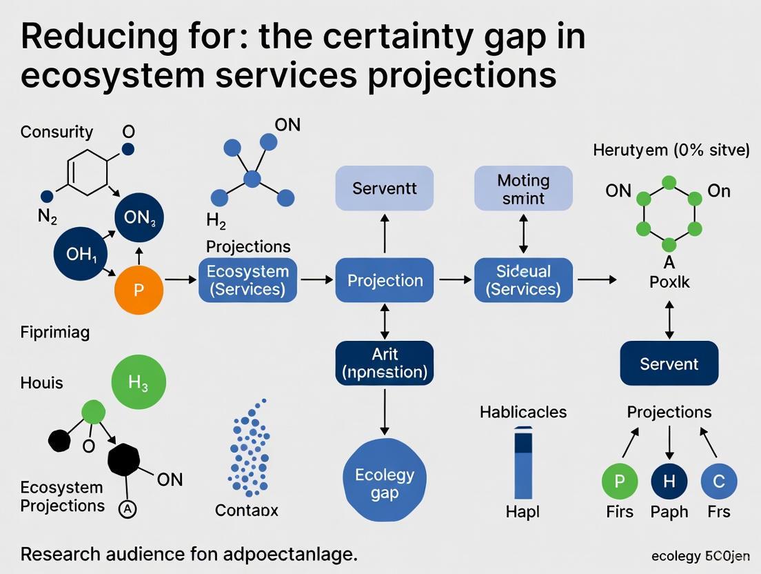
Closing the Certainty Gap: How Model Ensembles Are Revolutionizing Ecosystem Services Projections
This article addresses the critical 'certainty gap' in ecosystem services (ES) modeling—the uncertainty about model accuracy that hinders their use in decision-making.
Closing the Certainty Gap: How Model Ensembles Are Revolutionizing Ecosystem Services Projections
Abstract
This article addresses the critical 'certainty gap' in ecosystem services (ES) modeling—the uncertainty about model accuracy that hinders their use in decision-making. We explore how model ensembles, which combine multiple individual models, are emerging as a powerful solution to reduce uncertainty and increase the reliability of projections for services like water supply and carbon storage. Tailored for researchers and development professionals, the content covers the foundational concepts of ES uncertainty, methodological guidance for building weighted and unweighted ensembles, strategies for troubleshooting common pitfalls, and validation techniques demonstrating 2–14% accuracy gains. The synthesis provides a robust framework for integrating these approaches into environmental research and policy design to support sustainable development goals.
Understanding the Certainty Gap: Why Single Ecosystem Service Models Fall Short
Defining the 'Certainty Gap' and 'Capacity Gap' in Ecosystem Services Assessment
Frequently Asked Questions
What is the "Certainty Gap" in ecosystem services assessment? The Certainty Gap refers to the lack of knowledge about the accuracy of available ecosystem service models. This makes it difficult for practitioners to know which model to trust for decision-making, as model projections can be highly variable. This gap undermines confidence in the projections from these models [1] [2].
What is the "Capacity Gap" in ecosystem services assessment? The Capacity Gap is the lack of access to ES models, data, computational power, and technical expertise needed to implement them. This includes barriers like funds for software, person-time to learn complex systems, and access to high-quality input data. This gap is typically more substantial in poorer nations and regions [1].
Why are these gaps a significant problem for research and policy? These gaps are interconnected and create a significant barrier to using ecosystem science in policy and decision-making. The Capacity Gap prevents researchers from generating information, while the Certainty Gap reduces the confidence in the information that is produced. This can lead to either the selection of a suboptimal model, potentially causing poor decisions, or a complete reluctance to use ES models altogether [1] [3] [2].
What is a model ensemble and how can it help? A model ensemble is the combination of multiple individual models to produce a single, more robust output. Instead of relying on one model, an ensemble uses the median or mean value from several models for each location. Research shows that ensembles are consistently 2% to 14% more accurate than any single model chosen at random and provide a way to quantify uncertainty [1] [2].
Are some ensemble methods better than others? Yes. While a simple unweighted average (committee averaging) of models improves accuracy, more sophisticated weighted ensembles generally provide even better predictions. Weighted ensembles assign different levels of influence to each model based on its accuracy or consensus with other models [1] [2].
Besides ensembles, what other approaches can reduce these gaps? Other strategies include developing and adopting standardized uncertainty assessment protocols across ES studies [3] and creating integrative frameworks like the ecosystem capacity index, which better links ecosystem condition accounts to the capacity for supplying specific services [4].
Troubleshooting Guides
Guide 1: Addressing the Certainty Gap with Model Ensembles
Problem: A researcher or policy-maker is unsure which of many available ecosystem service models to use for a regional assessment and lacks the local data to validate the model's accuracy.
Solution: Implement a model ensemble approach.
Experimental Protocol: Creating a Weighted Ensemble
- Model Selection: Identify and run multiple available models for your target ecosystem service (e.g., carbon storage, water yield) for your region of interest. The number of models can range from 5 for recreation to 14 for carbon storage in global studies [1].
- Output Normalization: Process the raw model outputs to make them comparable. This often involves normalizing the values and correcting them on a per-area basis [2].
- Determine Model Weights:
- If validation data are available: Calculate the accuracy of each model against local independent data. Use statistical measures like deviance or Spearman's ρ. Weight each model's contribution to the final ensemble based on its accuracy [2].
- If no validation data are available (most common): Use a consensus-based weighting method. Models whose outputs are more different from the group (idiosyncratic) are given lower weights, reducing the impact of potential outliers [2].
- Calculate Ensemble Value: For each location (e.g., grid cell), calculate the final ensemble value. This can be the unweighted median or a weighted average based on the weights determined in the previous step.
- Validate and Communicate Uncertainty: Compare the final ensemble's accuracy against any available independent data. Use the variation among the individual models (e.g., standard error of the mean) as a proxy for uncertainty when communicating results [1].
Visualization: Ensemble Creation Workflow
Guide 2: Bridging the Capacity Gap with Open Data and Integrated Frameworks
Problem: A research team in a data-poor region lacks the computational resources, software licenses, or technical expertise to run multiple complex ecosystem service models.
Solution: Leverage freely available ensemble data and adopt simpler, integrated accounting frameworks.
Experimental Protocol: Implementing an Ecosystem Capacity Index
For situations where running complex models is not feasible, the Ecosystem Capacity Index offers an alternative method to link ecosystem condition to service delivery, based on the System of Environmental Economic Accounting (SEEA) framework [4].
- Develop Condition Account: Compile a set of biophysical indicators (e.g., tree height, soil organic matter, water quality) to assess the condition of an ecosystem asset relative to a reference state [4].
- Define Capacity Scores: For each ecosystem service of interest (e.g., timber provisioning, water filtration), assign a vector of capacity scores. Each score represents how a specific condition indicator influences the capacity to supply that service [4].
- Construct the Index: Combine the condition account with the capacity scores to derive a capacity index for each ecosystem asset and service. This reveals that an ecosystem with a fixed condition profile may have different capacities for supplying different services [4].
- Integrate with Services Accounts: Use the capacity index to better inform the ecosystem services accounts, creating a more rigorous connection between observed condition and estimated service supply [4].
Visualization: Capacity Index Framework
Quantitative Data on Ensemble Performance
The table below summarizes the demonstrated improvement in accuracy gained by using model ensembles over individual models for five key ecosystem services, as validated by independent data [1].
Table 1: Accuracy Improvement of Model Ensembles over Individual Models
| Ecosystem Service | Type of Service | Number of Models in Ensemble | Median Accuracy Improvement |
|---|---|---|---|
| Water Supply | Provisioning | 8 | 14% |
| Recreation | Cultural | 5 | 6% |
| Aboveground Carbon Storage | Regulating | 14 | 6% |
| Fuelwood Production | Provisioning | 9 | 3% |
| Forage Production | Provisioning | 12 | 3% |
Table 2: Essential Resources for Addressing Gaps in Ecosystem Services Assessment
| Resource / Tool | Type | Primary Function | Relevance to Gaps |
|---|---|---|---|
| Global ES Ensembles Dataset [1] | Data | Provides pre-computed ensemble values and accuracy estimates for 5 key ES at ~1km resolution. | Directly addresses both Capacity and Certainty gaps by providing free, ready-to-use, accuracy-assessed data. |
| Ecosystem Services Valuation Database (ESVD) [5] | Data | A global database of economic values for ES, standardized to common units. | Helps address the Capacity Gap by providing a central repository of economic values, reducing the need for primary valuation studies. |
| Weighted Ensemble Algorithms [2] | Methodology | Statistical methods (e.g., deterministic consensus, regression to median) for combining model outputs. | Reduces the Certainty Gap by providing a superior method for creating accurate ensemble predictions. |
| SEEA Ecosystem Accounting [4] | Framework | The international statistical standard for integrating environmental and economic data. | Provides a standardized structure for developing ecosystem condition and capacity accounts, reducing methodological uncertainty. |
| Uncertainty Assessment Framework [3] | Guidelines | Best practices for identifying, quantifying, and communicating uncertainties in ES assessments. | Directly targets the Certainty Gap by promoting transparency and robust handling of error and uncertainty. |
Troubleshooting Guides
Troubleshooting Guide 1: Diagnosing and Remedying Poor Model Generalization
Q: My model performs well on training data but fails on new, unseen data. What is happening and how can I fix it?
This issue typically indicates overfitting, where your model has learned the noise in the training data rather than the underlying pattern. Follow this diagnostic workflow to identify and remedy the specific cause.
Experimental Protocol: Bias-Variance Diagnosis via Learning Curves
- Objective: Quantitatively diagnose overfitting (high variance) or underfitting (high bias) by plotting model performance against increasing training set sizes.
- Materials: See "Research Reagent Solutions" table.
- Procedure:
- Split your dataset into training and validation sets using a 70-30 ratio.
- Train your model on incrementally larger subsets of the training data (e.g., 10%, 20%, ..., 100%).
- For each training subset, calculate and record the model's performance score (e.g., RMSE for regression, F1-score for classification) on both the training subset and the fixed validation set.
- Plot the learning curves: training score and validation score (y-axis) against training set size (x-axis).
- Interpretation:
- Overfitting: Training score remains significantly higher than validation score, and the validation score may plateau without improving.
- Underfitting: Both training and validation scores are low and converge to a similar, unsatisfactory value.
Remedial Actions Based on Diagnosis:
| Diagnosis | Primary Cause | Remedial Actions | Key Metrics to Monitor |
|---|---|---|---|
| Overfitting [6] [7] | Model too complex for available data | - Increase training data- Apply regularization (L1/L2)- Reduce model complexity (e.g., prune trees, reduce layers)- Use feature selection to remove noise | - Gap between training/validation accuracy narrowing- Improved F1-score on validation set |
| Underfitting [6] [7] | Model too simple to capture patterns | - Add relevant features or create interaction terms- Use a more complex model (e.g., switch from linear to tree-based)- Reduce regularization- Improve feature engineering | - Increase in training accuracy- Improved recall and precision |
| Data Quality Issues [8] [9] | Foundational data problems | - Impute missing values (median, KNN)- Handle outliers (winsorization)- Standardize formats and scales | - Decreased RMSE after preprocessing- More balanced class distribution |
Troubleshooting Guide 2: Selecting the Right Model for Ecosystem Services Research
Q: With many algorithms available, how do I systematically choose the best model for predicting ecosystem services to reduce the "certainty gap"?
The "certainty gap" refers to the lack of knowledge about model accuracy, particularly acute in data-poor regions [10] [11]. A systematic selection process is crucial for reliable, actionable predictions.
Experimental Protocol: Model Evaluation via k-Fold Cross-Validation
- Objective: To obtain a reliable estimate of model performance and generalization error, reducing the "certainty gap."
- Materials: Preprocessed dataset, candidate machine learning algorithms.
- Procedure:
- Randomly shuffle the dataset and split it into k equal-sized folds (common choices are k=5 or k=10).
- For each candidate model, perform the following k times:
- Designate one fold as the validation set and the remaining k-1 folds as the training set.
- Train the model on the training set.
- Evaluate the model on the validation set and record the chosen performance metric(s).
- Calculate the average performance metric across all k folds for each model.
- Select the model with the best average performance, or proceed to build an ensemble.
Model Selection Guide Based on Data and Task:
| Task / Data Characteristic | Recommended Initial Models | Rationale & Consideration |
|---|---|---|
| Tabular Data (e.g., species count, soil properties) | Random Forest, Gradient Boosting (XGBoost) [12] [9] | Handles mixed data types and non-linear relationships well. Strong performance on structured data. |
| Spatial Data (e.g., satellite imagery, habitat maps) | Convolutional Neural Networks (CNNs) [12] | Excellently captures spatial patterns and hierarchies in image data. |
| Small Datasets (< 1,000 samples) | Logistic/Linear Regression, Shallow Decision Trees [12] | Less prone to overfitting. Provides a strong, interpretable baseline. |
| High Interpretability Required (e.g., policy guidance) | Linear Models, Decision Trees [13] [14] | Decisions are easier to trace and explain to stakeholders, crucial for building trust. |
| Maximizing Predictive Accuracy | Model Ensembles (e.g., Random Forest, Stacking) [10] [11] | Combining multiple models can increase accuracy by 2-14% and provides more robust, reliable projections, directly addressing the certainty gap. |
Frequently Asked Questions (FAQs)
Q1: What are the most common mistakes in model selection for applied research projects?
The most frequent pitfalls include [7]:
- Chasing complex models first: Starting with deep learning before establishing a simple baseline, which wastes resources and can lead to overfitting on smaller datasets.
- Misplaced metric focus: Optimizing for overall accuracy on imbalanced datasets (e.g., where rare species or disease cases are the critical class) instead of using precision, recall, or F1-score.
- Data leakage: Preprocessing or feature engineering on the entire dataset before splitting into training and test sets, resulting in over-optimistic performance estimates.
- Ignoring model assumptions: Applying models without checking if their underlying assumptions (e.g., linearity, normality) are met by the data.
- Neglecting the "big picture": Selecting a model based solely on technical metrics while ignoring operational constraints like computational cost, interpretability for stakeholders, and deployment environment [13] [14].
Q2: How can I be sure my chosen model will perform well in production?
Beyond cross-validation, implement these strategies:
- Test on real-world pilot data: Create a staging environment where the model processes live or recently acquired data to monitor for performance drops due to concept drift or data shifts [6].
- Track stability and latency: Monitor not just accuracy, but also inference time and resource usage to ensure the model meets operational requirements [6] [14].
- Use champion-challenger frameworks: Deploy your new model alongside the existing one (if any) in a controlled manner, comparing their performance on a small fraction of real-world traffic before full rollout.
Q3: My dataset is small and from a data-poor region. Can I still build a reliable model?
Yes. Model ensembles are particularly valuable here. Research on global ecosystem service models has shown that ensembles of multiple models provide 2-14% more accurate predictions than individual models. Crucially, this accuracy is distributed equitably across the globe, meaning countries with less research capacity do not suffer an accuracy penalty, thereby directly reducing the "capacity and certainty gaps" [10] [11]. Other techniques include:
- Transfer Learning: Using a pre-trained model on a large, general dataset and fine-tuning it on your specific, smaller dataset.
- Data Augmentation: Artificially creating new training examples from existing ones (e.g., rotating images, adding noise).
- Simpler Models: Prioritizing robust, interpretable models that are less likely to overfit on limited data.
The Scientist's Toolkit: Research Reagent Solutions
| Tool / Reagent | Function / Purpose | Example Use-Case in Ecosystem Research |
|---|---|---|
| Scikit-learn [14] | Provides a unified library for baseline models, feature selection, cross-validation, and hyperparameter tuning. | Rapid prototyping of multiple model candidates (e.g., SVM, Random Forest) for species distribution modeling. |
| XGBoost / LightGBM [9] | High-performance gradient boosting frameworks ideal for structured/tabular data. Often achieves state-of-the-art results. | Predicting forest carbon stocks from tabular data on tree measurements, soil properties, and climate variables. |
| SHAP (SHapley Additive exPlanations) [6] | Explains the output of any ML model, quantifying the contribution of each feature to a specific prediction. | Interpreting a complex model to understand which environmental drivers (e.g., precipitation, temperature, slope) most influence habitat suitability. |
| Optuna / Hyperopt [9] | Frameworks for automated hyperparameter optimization, using efficient search algorithms like Bayesian optimization. | Systematically tuning the hyperparameters of a neural network to maximize its accuracy in land cover classification from satellite imagery. |
| K-Fold Cross-Validation [6] [12] [14] | A resampling technique used to assess model generalizability and reduce overfitting. | Providing a robust performance estimate for a model predicting water quality, ensuring it works across different geographic subsets of the data. |
Troubleshooting Guide: Frequently Asked Questions
FAQ 1: Why is uncertainty assessment (UA) critical in ecosystem services (ES) research, and what are the common challenges? Uncertainty assessment is essential because omitting it limits the validity of findings and can undermine the 'science-based' decisions they inform. Despite its importance, UA often receives superficial treatment due to several common challenges [3]. These include the perceived technical difficulty of conducting UA, concerns about the utility of UA for decision-makers, and a lack of practical tools and guidelines tailored to the interdisciplinary nature of ES science [3].
FAQ 2: How significant is the uncertainty from ecological models compared to climate models? Uncertainty associated with species distribution models (SDMs) can be substantial and can even exceed the uncertainty generated from diverging earth system models (climate models). In some projections, SDM uncertainty can account for up to 70% of the total uncertainty by the year 2100 [15]. This result has been found to be consistent across species with different functional traits.
FAQ 3: How does projecting into novel environmental conditions affect model performance? Model performance degrades, and uncertainty increases, when models extrapolate into novel environmental conditions outside the range of their training data [15]. The predictive power of species distribution models remains relatively high in the first 30 years of projections but becomes less certain over longer time horizons as environmental novelty increases [15].
FAQ 4: What are the primary sources of uncertainty in ES projections? Uncertainty propagates from multiple sources within a projection framework. The main categories are [15]:
- Ecological Model Uncertainty: Arises from differences in model type, design, and parameterization, as well as from imperfect sampling of the ecosystem.
- Earth System Model (Climate) Uncertainty: Stems from using different climate models and future emission scenarios.
- Scenario Uncertainty: Related to different pathways of future forcing variables, like greenhouse gas emissions.
- Observation Uncertainty: Introduced by biases in data that inadequately capture the full environmental niche of a species.
FAQ 5: How can researchers begin to quantify and reduce uncertainty? A key recommendation is to use ensembles of models rather than relying on a single model type [15]. Furthermore, adopting best practices and insights from integrated assessment communities, which have a long history of dealing with interdisciplinary modeling, can directly improve ES assessments [3]. Utilizing simulated species distributions (virtual species) provides a known "truth" against which model performance and uncertainty can be systematically evaluated [15].
Quantitative Data on Uncertainty in Species Distribution Projections
Table 1: Summary of Key Quantitative Findings on Projection Uncertainty from a Simulation Study [15]
| Uncertainty Factor | Key Finding | Notes |
|---|---|---|
| SDM vs. ESM Uncertainty | SDM uncertainty can contribute up to 70% of total uncertainty by 2100. | Finding was consistent across different species traits. |
| Temporal Horizon | SDM uncertainty increases through time. | Predictive power is relatively higher in the first 30 years, aligning with strategic decision-making timelines. |
| Environmental Extrapolation | SDM uncertainty is primarily related to the degree models extrapolate into novel environmental conditions. | Uncertainty is moderated by how well models capture the underlying dynamics of species distributions. |
Table 2: Key Drivers of Global Ecosystem Service Supply-Demand Relationships (2000-2020) [16]
| Driver | Ecosystem Service Most Affected | Mean Contribution Rate | Nature of Influence |
|---|---|---|---|
| Human Activity | Food Production | 66.54% | Primary shaping force |
| Human Activity | Carbon Sequestration | 60.80% | Primary shaping force |
| Climate Change | Soil Conservation | 54.62% | Greater controlling force |
| Climate Change | Water Yield | 55.41% | Greater controlling force |
Experimental Protocols for Key Methodologies
Protocol 1: A Framework for Quantifying Uncertainty Using Virtual Species
This protocol is designed to systematically evaluate Species Distribution Model (SDM) performance and isolate sources of uncertainty using a known simulated truth [15].
- Define Species Archetypes: Create simplified representations of species groups with different functional traits and ecological preferences (e.g., Highly Migratory Species, Coastal Pelagic Species, Groundfish Species) [15].
- Simulate "True" Distributions: Use a combination of regional ocean climate projections and a species distribution simulation tool (e.g., as described in Leroy et al., 2016) to generate spatially explicit biomass data for each archetype from 1985-2100. This simulated data serves as the validation benchmark [15].
- Train Ensemble of SDMs: Fit a diverse ensemble of SDMs (e.g., 15 different model types) to the simulated biomass data for a historical training period (e.g., 1985-2010) [15].
- Project Future Distributions: Project each SDM from the end of the training period into the future (e.g., 2011-2100) using an ensemble of regional climate models (e.g., 3 different models) [15].
- Quantify Uncertainty: Compare the output of all SDM projections against the simulated "true" distributions for the projection period. Quantify the uncertainty introduced by the climate projection (ESM uncertainty) and the ecological modeling (SDM uncertainty) [15].
Protocol 2: Assessing Global Ecosystem Service Supply and Demand (ESSD)
This protocol outlines a pixel-scale approach for assessing the balance between ecosystem service supply and demand over a continuous time series [16].
- Data Collection and Pre-processing:
- Gather global datasets for land use, NDVI, soil, temperature, precipitation, population, and food production.
- Resample all datasets to a consistent spatial resolution (e.g., 1x1 km) [16].
- Calculate Ecosystem Service Supply:
- Food Production: Estimate via a linear relationship between land use category yield and NDVI [16].
- Carbon Sequestration: Calculate based on photosynthesis principles, using Net Primary Productivity (NPP) data [16].
- Soil Conservation: Define as the difference between potential and actual soil erosion, estimated with the Revised Universal Soil Loss Equation (RUSLE) [16].
- Water Yield: Derive from the water balance equation and convert to volume based on raster area [16].
- Calculate Ecosystem Service Demand:
- Analyze ESSD Relationships and Drivers:
- Map spatial and quantitative matching relationships between supply and demand.
- Use statistical methods (e.g., geographical detector models) to quantify the impacts and contribution rates of climate change and human activities on the ESSD relationships [16].
Visualizing Uncertainty in Ecosystem Services Research
Diagram 1: Uncertainty Propagation in Ecosystem Service Projections
Diagram 2: Virtual Species Validation Workflow
Table 3: Essential Resources for Ecosystem Services and Uncertainty Research
| Resource/Solution | Function/Description | Example Use Case |
|---|---|---|
| Ensemble Modeling | Using multiple model types/structures to capture a range of plausible outcomes and quantify model-based uncertainty. | Quantifying SDM vs. ESM uncertainty in species distribution projections [15]. |
| Virtual Species | Simulated species with predefined environmental responses, providing a known "truth" for model validation. | Experimental testing and developing best-practice principles for SDMs [15]. |
| Global ES & Biodiversity Maps | High-spatial-resolution, open-source models mapping ecosystem services and biodiversity metrics. | Quantifying the direct impact of corporate assets or other drivers on nature [17]. |
| Pixel-Scale Analysis | Assessing ES supply and demand at the pixel level (e.g., 1x1 km) to precisely capture spatial patterns and changes. | Analyzing global ESSD dynamics over long time series [16]. |
| RUSLE (Revised Universal Soil Loss Equation) | An empirical model used to estimate rates of soil erosion caused by rainfall and associated overland flow. | Calculating soil conservation supply as the difference between potential and actual erosion [16]. |
| SALSA Framework | A systematic methodology (Search, Appraisal, Synthesis, Analysis) for conducting rigorous literature reviews. | Reviewing progress in specific ES research fields, like regulating services [18]. |
| Regional Climate Downscaling | Using higher-resolution models to dynamically or statistically downscale global climate projections. | Capturing fine-scale environmental variability for regional species distribution projections [15]. |
Technical Support Center
Troubleshooting Guide
This guide addresses common issues encountered when modeling the water provision ecosystem service.
Table 1: Troubleshooting Common Problems in Water Provision Mapping
| Problem Scenario | Potential Causes | Diagnostic Checks | Recommended Solutions |
|---|---|---|---|
| Drastic changes in output when altering spatial resolution (e.g., from 30m to 300m). | Modifiable Areal Unit Problem (MAUP); loss of small, critical land cover features (e.g., wetlands) at coarser resolutions [19]. | Compare land cover class distributions at different resolutions. Check if small, high-value patches are aggregated out [19]. | Use the finest resolution data feasible. Conduct a multi-scale analysis to identify critical scale thresholds for your study area [19]. |
| Significant discrepancies in annual water yield totals when using different temporal scales (e.g., annual vs. seasonal models). | Model does not capture seasonal climate variations (e.g., distinct wet/dry seasons), leading to inaccurate runoff and recharge estimates [20]. | Compare monthly precipitation and evapotranspiration data. Run a seasonal water yield model to check for improvements [20]. | Use a seasonal water yield model instead of an annual model in regions with strong seasonal climate patterns [20]. |
| Spatial pattern of water provision is highly sensitive to a few input parameters. | High model sensitivity to specific biophysical parameters; may indicate equifinality or over-reliance on a single calibrated value [21]. | Perform a global sensitivity analysis to identify parameters that most influence key outputs (e.g., baseflow, quickflow) [21]. | Calibrate the model using decision-relevant metrics (e.g., targeting low flows or flood flows) instead of general performance metrics [21]. |
| Model performs well at the watershed outlet but poorly in ungauged sub-basins. | Parameters were screened and calibrated only for a single, gauged location, missing spatial variations in controlling processes [21]. | Evaluate parameter sensitivity at multiple, distributed locations (e.g., hillslope outlets), not just the main outlet [21]. | Implement a spatially distributed sensitivity analysis and calibration where possible, or use parameter multipliers that are informed by local physical characteristics [21]. |
| Uncertainty from different data sources (e.g., soil or LULC maps) leads to vastly different conclusions. | Underlying classifications and accuracy of spatial datasets vary, propagating uncertainty through the model [22] [20]. | Quantify uncertainty by running the model with multiple credible datasets for the same input [22]. | Use the most locally accurate and recent data available. Report results as a range from multiple scenarios to communicate uncertainty to decision-makers [22] [20]. |
Frequently Asked Questions (FAQs)
Q1: Why does the spatial resolution (grain size) of my input data so drastically change my water yield estimates? The effect of changing spatial resolution is a classic geographic issue known as the Modifiable Areal Unit Problem (MAUP) [19]. When you aggregate data to a coarser resolution:
- Information is lost: Small, discrete land cover types that are critical for hydrology (e.g., a small wetland or a patch of forest) can be "averaged out" or merged into a dominant surrounding class [19]. One study found that using fine-resolution (30 m) data could yield ecosystem service values 198% greater than those derived from coarse-resolution (1 km) data for this reason [19].
- Spatial patterns are homogenized: The landscape becomes statistically smoother, reducing variance and altering the perceived spatial structure of ecosystem services [19].
Q2: My model is calibrated perfectly at the main river gauge, but why are the predictions for upstream sub-catchments so unreliable? This is a common challenge. Calibration at a single, aggregated location (like a watershed outlet) often leads to equifinality—where multiple different parameter sets can produce similarly good results at that one point [21]. However, these parameter sets may simulate very different hydrological processes in ungauged upstream areas [21]. The solution is to move beyond outlet-only calibration by:
- Using decision-relevant sensitivity metrics evaluated at the spatial scales of interest for your management questions [21].
- Screening parameters based on their influence on hydrological processes in hillslopes and sub-catchments, not just at the outlet [21].
Q3: How can I quantify and communicate the uncertainty in my water provision maps to decision-makers? Ignoring uncertainty reduces the reliability of your maps for decision-making [22] [20]. We recommend a scenario-based approach to uncertainty assessment:
- Explicitly model different sources of uncertainty by creating multiple scenarios. Key sources include [22] [20]:
- Spatial Data: Run your model with different LULC or soil maps.
- Modeling Scales: Test different spatial resolutions and temporal scales (e.g., annual vs. seasonal).
- Parameterization: Use parameter values from different literature sources or expert opinions.
- Present your results as a range (e.g., maps of minimum, maximum, and median estimates) rather than a single map. This visually communicates robustness and identifies areas where conclusions are highly uncertain [20].
Q4: What is the practical difference between using an annual water yield model and a seasonal water yield model? The choice is critical in landscapes with seasonal climates. An annual model sums water provision over the entire year, which can mask critical intra-annual variations [20]. A seasonal model:
- Separates water yield into quick flow (storm runoff), local recharge, and base flow (sustained streamflow from groundwater) [20].
- Provides more accurate and actionable information for managing water resources during dry seasons (relying on baseflow) and for mitigating flood risk during wet seasons (understanding quick flow) [20].
Experimental Protocols & Data
Detailed Methodology: Uncertainty Assessment for Water Provision Mapping
This protocol is adapted from the Fitzroy Basin case study [20] and related research on scale effects [19].
1. Define the Baseline Scenario
- Model Selection: Choose a spatially explicit water yield model (e.g., the InVEST Seasonal Water Yield Model).
- Data Preparation: Assemble the best available data for your region to establish a baseline. Core data needs include:
- Digital Elevation Model (DEM): A high-resolution DEM (e.g., 30 m SRTM-derived) for defining watersheds and flow paths.
- Land Use/Land Cover (LULC): A recent, locally validated LULC map.
- Climate Data: Long-term monthly precipitation and reference evapotranspiration data from reliable weather stations or databases.
- Soil Data: A map of hydrologic soil groups (HSG) based on saturated hydraulic conductivity.
- Parameterization: Assign biophysical parameters (e.g., runoff curve numbers, crop coefficients (Kc)) using validated local sources, literature, or hydrological software.
2. Design and Execute Uncertainty Scenarios Systematically alter the baseline inputs and model structure as summarized in the table below.
Table 2: Experimental Design for Assessing Uncertainty in Water Provision Estimates [22] [19] [20]
| Uncertainty Source | Variable Tested | Scenario Examples | Key Quantitative Metrics for Comparison |
|---|---|---|---|
| Spatial Scale | Data Resolution | Run the model at 30 m, 100 m, and 300 m resolutions. | Total annual water yield (km³/yr); Spatial pattern similarity (e.g., Moran's I); Area of high-value provisioning patches. |
| Temporal Scale | Model Structure | Compare an Annual Water Yield model with a Seasonal Water Yield model. | Quick flow, local recharge, and base flow volumes; Model performance during wet vs. dry seasons. |
| Parameterization | Biophysical Parameters | Use high, medium, and low values for key parameters (e.g., Curve Number, Kc) from different literature sources. | Annual totals of water yield and base flow; Sensitivity indices (e.g., from a global sensitivity analysis). |
| Spatial Data Source | Input GIS Layers | Use different LULC maps (e.g., from different years or classification schemes). | Difference in spatial distribution of water yield; Change in ranked importance of sub-watersheds. |
3. Analyze and Compare Outputs
- Quantify differences in both the magnitude (total water yield) and spatial pattern of water provision across the scenarios.
- Use statistical and spatial metrics (see Table 2) to compare the outputs against the baseline.
- Identify areas of the landscape where conclusions about water provision are robust (i.e., consistent across scenarios) and areas where they are highly uncertain.
Workflow Visualization
The following diagram illustrates the logical workflow for conducting an uncertainty assessment in water provision mapping.
The Scientist's Toolkit
Table 3: Essential Research Reagents and Data Solutions for Water Provision Mapping
| Item Name | Function / Role in the Experiment | Key Considerations for Selection |
|---|---|---|
| Spatially Explicit Hydrological Model | The core engine for calculating water flux and storage across a landscape. Examples: InVEST, RHESSys, SWAT. | Choose based on process representation (e.g., seasonal vs. annual), data requirements, and compatibility with your study's spatial and temporal scales [20] [21]. |
| Land Use/Land Cover (LULC) Map | Determines key biophysical parameters (e.g., evapotranspiration, infiltration) for each pixel, driving the hydrological simulation [20]. | Prioritize locally validated, recent maps. Be aware that differences in classification schemes between datasets are a major source of uncertainty [22] [19]. |
| Digital Elevation Model (DEM) | Defines the topography-driven physical structure of the watershed, including flow accumulation, stream networks, and slope [20]. | Higher resolution (e.g., 30m SRTM) generally provides more accurate watershed delineation and flow routing than coarser models [20]. |
| Hydrologic Soil Groups (HSG) | Classifies soil types based on runoff potential (from low A to high D), which is critical for calculating infiltration and runoff [20]. | Derived from soil texture and hydraulic conductivity data. Accuracy depends on the source soil map's scale and classification method. |
| Global Sensitivity Analysis (GSA) | A computational "reagent" used to identify which model parameters have the greatest influence on your outputs, guiding effective calibration [21]. | Use decision-relevant metrics (e.g., sensitivity of low flows) for screening, not just general model performance metrics. Should be evaluated at multiple spatial scales [21]. |
Building Better Predictions: A Practical Guide to Model Ensembles
Frequently Asked Questions (FAQs)
1. What is the core principle behind error reduction in ensemble modeling? The core principle is that by combining the predictions from multiple models, their individual errors "average out" [23]. This aggregation reduces the overall variance of the predictions without increasing bias, a concept known as the bias-variance tradeoff [23] [24] [25]. The combined output is typically more accurate and robust than any single model's output [23] [26].
2. Why is model diversity crucial in an ensemble? Diversity is key because combining several models that all make the same error provides no benefit [24] [26]. If the models are independent and their errors are uncorrelated, then the error of the ensemble can be significantly lower than the average error of the individual models [24]. Diversity can be achieved by using different algorithms, different subsets of training data, or different model parameters [24] [25].
3. My ensemble is not performing better than my best base model. What could be wrong? This is often a sign of insufficient diversity among your base models [24] [26]. If all your models are highly correlated and make similar errors, the ensemble cannot correct them. To fix this, ensure diversity by:
- Using different model types (e.g., decision trees, neural networks) [26].
- Training models on different bootstrap samples of your data (Bagging) [25].
- Varying key hyperparameters or initial conditions for each model [23].
4. How do I choose between averaging and weighted averaging for my ensemble? Simple averaging treats all models as equally competent and is a robust default choice [23] [27]. Weighted averaging assigns higher influence to models that demonstrate better performance (e.g., lower error on a validation set) [23] [27]. Weighted averaging is beneficial when you have clear evidence that some models are consistently more reliable than others [23].
5. What are the common computational challenges with ensemble modeling? The primary challenge is resource intensity. Training and maintaining multiple models instead of one increases demands on:
- Computational Time and Power: Training can be slow and requires more processing capacity [28] [26].
- Memory: Storing multiple models consumes more memory [26]. Strategies to mitigate this include using architectures that share common base layers [28] and parallelizing training where possible [24] [25].
Troubleshooting Guides
Issue: Ensemble Shows High Variance and Overfits
- Symptoms: The ensemble performs excellently on training data but poorly on unseen test data or validation data.
- Possible Causes and Solutions:
- Cause 1: Base models are themselves overfitting and are too complex.
- Cause 2: The ensemble is not large enough to average out the noise.
- Solution: Increase the number of base models in the ensemble. Research shows that increasing the number of models (M) can reduce the ensemble error [24].
Issue: Ensemble Shows High Bias and Underfits
- Symptoms: Performance is poor on both training and test data.
- Possible Causes and Solutions:
- Cause 1: The base learners are too weak (e.g., very simple models).
- Cause 2: The models are not capturing the underlying patterns in the data.
- Solution: Perform feature engineering to provide more informative inputs to your models.
Issue: Ensemble Performance is Saturated or Degrading with Added Models
- Symptoms: Adding more models to the ensemble provides no improvement or even hurts performance.
- Possible Causes and Solutions:
Experimental Protocols and Data
Protocol 1: Implementing a Basic Averaging Ensemble
This protocol outlines the steps to create a simple yet effective ensemble for regression or classification.
- Base Model Selection: Choose your base learning algorithms (e.g., Linear Regression, Decision Trees, Support Vector Machines). For diversity, use different algorithms [26].
- Generate Diverse Models: Create N instances of your base models. Diversity can be induced by:
- Train Models: Train each of the N models independently on their respective data [23].
- Aggregate Predictions:
Protocol 2: A Species Distribution Model (SDM) Ensemble for Ecosystem Projections
This protocol is adapted from a study quantifying uncertainty in ecosystem services projections [15]. It demonstrates a real-world application of ensemble modeling to reduce the "certainty gap."
- Objective: Project future species distributions under climate change while quantifying uncertainty.
- Experimental Workflow:
- Input Data Preparation: Gather historical species occurrence data and environmental covariates (e.g., sea surface temperature, salinity).
- Earth System Model (ESM) Ensemble: Obtain future environmental projections from an ensemble of multiple ESMs to account for climate uncertainty.
- Species Distribution Model (SDM) Ensemble: Fit an ensemble of different SDM types (e.g., Generalized Additive Models, Random Forests) to the historical data.
- Cross-Projection: Project each SDM using the environmental outputs from each ESM, creating a matrix of projections.
- Uncertainty Quantification: Analyze the variance in projections across the SDM ensemble to identify areas and time periods with high epistemic uncertainty.
Table 1: Key Findings from an SDM Ensemble Study on Uncertainty Sources [15]
| Uncertainty Source | Description | Contribution to Total Uncertainty |
|---|---|---|
| Species Distribution Model (SDM) Uncertainty | Differences in model type, design, and parameterization. Can exceed 70% of total uncertainty by 2100. | Up to 70% |
| Earth System Model (ESM) Uncertainty | Differences in climate projections from various global climate models. | Varies, less than SDM uncertainty |
| Scenario Uncertainty | Differences arising from future emission scenarios (e.g., RCPs). | Not quantified in study |
| Internal Variability | Natural, unpredictable fluctuations in the climate system. | Not quantified in study |
Protocol 3: Advanced Architecture for Efficient Ensembles
For researchers concerned about the computational cost of traditional ensembles, the Divergent Ensemble Network (DEN) offers a more efficient architecture [28].
- Shared Base: A common set of initial layers processes the input data to learn a shared representation.
- Independent Branching: The network then diverges into multiple independent branches. Each branch has its own weights and acts as a separate model in the ensemble.
- Training: Branches are trained independently to maintain diversity in their predictions.
- Output: Predictions from all branches are averaged for the final output.
Result: This architecture reduces parameter redundancy and computational time (one study reported a 6x improvement in inference time) while maintaining the uncertainty estimation benefits of a full ensemble [28].
The Scientist's Toolkit: Research Reagent Solutions
Table 2: Essential Computational Tools for Ensemble Modeling
| Tool / Resource | Function | Example Use Cases |
|---|---|---|
| Scikit-learn (Python) | Provides easy-to-use implementations of Bagging, Random Forests, and Voting ensembles. | Rapid prototyping of bagging and stacking ensembles for classification and regression. |
| XGBoost (Python/R) | An optimized library for gradient boosting, a powerful sequential ensemble method. | Winning data science competitions; handling imbalanced data and complex nonlinear relationships. |
| LightGBM (Python/R) | Another high-performance gradient boosting framework, often faster than XGBoost. | Training on large-scale datasets with high-dimensional features. |
| Random Forest | A bagging ensemble of decorrelated decision trees. | A robust, all-purpose model that provides feature importance estimates. |
| TensorFlow/PyTorch | Deep learning frameworks for building custom neural network ensembles and advanced architectures like DENs. | Implementing custom ensemble layers, shared-base networks, and Bayesian deep learning ensembles. |
Committee averaging, also known as ensemble averaging, is a foundational machine learning technique where multiple models (often referred to as "experts" or "committee members") are combined to produce a single, more robust output. Unlike weighted approaches, the unweighted ensemble method assigns equal importance to each model's prediction, typically by calculating the mean for regression problems or the mode (majority vote) for classification tasks [23] [29]. In the context of ecosystem services (ES) research, this approach is increasingly valuable for reducing uncertainty in projections, as it mitigates the idiosyncratic errors and biases inherent in any single modeling framework [2]. By harnessing the "wisdom of the crowd" from multiple models, committee averaging provides a more stable and reliable foundation for critical environmental decision-making.
Core Concepts and Key Algorithms
Theoretical Foundation
The power of committee averaging rests on a few key principles:
- Bias-Variance Trade-off: Individual models can often be tuned for low bias at the cost of high variance. Combining several such high-variance models through averaging results in a final model that achieves both low bias and low variance, effectively resolving this fundamental trade-off [23].
- Error Reduction: When models' errors are uncorrelated, they tend to "average out" in the final committee prediction. Theoretically, if you have
Mindependent models, each with an error ofε, the error of the averaged committee can be reduced to approximatelyε / sqrt(M)[29]. - Diversity is Key: The success of an ensemble depends on the diversity of its constituent models. If all models make the same errors, averaging will not yield improvement. Diversity can be introduced by varying the training data, model algorithms, feature sets, or initial parameters [29].
Common Committee Averaging Algorithms in Practice
Different software and research communities implement committee averaging under various names and with slight variations. The table below summarizes key algorithms relevant to ecosystem modeling.
Table 1: Common Committee Averaging Algorithms
| Algorithm Name | Primary Application | Brief Description | Example Context |
|---|---|---|---|
| Committee Averaging (EMca) | Classification | Converts model outputs to binary (0/1) predictions and calculates the average vote [30] [31]. | biomod2 ensemble modeling [30]. |
| Ensemble Mean (EMmean) | Regression / Probability | Calculates the simple arithmetic mean of all model predictions (e.g., probabilities) [30] [31]. | biomod2 ensemble modeling [30]. |
| Ensemble Median (EMmedian) | Regression / Probability | Calculates the median of all model predictions, making the output more robust to outliers [30] [31]. | biomod2 ensemble modeling [30]. |
| Majority Voting | Classification | The class label that receives more than half the votes is selected. If no majority, it may result in no decision [29]. | General machine learning committees [29]. |
| Plurality Voting | Classification | The class label that receives the most votes (even if not a majority) is selected [29]. | General machine learning committees [29]. |
The following diagram illustrates the logical workflow and data flow in a standard committee averaging system, showing how diverse models are combined into a final, averaged output.
Frequently Asked Questions (FAQs)
Q1: Why should I use committee averaging instead of simply selecting the best-performing single model?
Empirical studies, particularly in ecosystem services, show that no single model is consistently the most accurate across different regions or validation datasets. While the "best" model can vary, the average accuracy of an ensemble is consistently higher than that of the average individual model. Ensembles smooth out extreme errors and provide a more conservative and reliable estimate, which is crucial for reducing the certainty gap in projections used for policy-making [2].
Q2: My ensemble model failed with an error stating "No models kept due to threshold filtering." What does this mean?
This error occurs in platforms like biomod2 when the evaluation scores of all your individual models fall below the threshold you set for inclusion in the ensemble (e.g., via the metric.select.thresh parameter). The function then has no models to average. To resolve this, you can:
- Lower your quality threshold to be less strict.
- Check the performance of your individual models to ensure they are reasonably accurate.
- Remove the threshold filter entirely by setting
metric.select.thresh = NULL, which will include all models in the committee average regardless of their score [32] [30].
Q3: How many models should I include in my committee?
There is no fixed rule, but the law of diminishing returns applies. Starting with a committee of 5-10 diverse models often yields significant benefits. The key is to prioritize model diversity over sheer quantity. Using different model types (e.g., GAM, GLM, Random Forest) and training them on different data subsets (e.g., via cross-validation) is more effective than having many very similar models [23] [29].
Q4: Is committee averaging only useful for species distribution models?
No, committee averaging is a universal method. While frequently used in species distribution modeling (e.g., via biomod2), it is equally applicable to a wide range of ecological and ecosystem service models, including water supply and carbon storage projections [2]. Furthermore, its utility extends to other fields, such as mitigating hardware-level errors in physical neural network implementations [33].
Troubleshooting Guide
Table 2: Common Issues and Solutions for Implementing Committee Averaging
| Problem | Possible Cause | Solution | Related Platform |
|---|---|---|---|
| "No models kept due to threshold filtering" | The metric.select.thresh value is set too high, excluding all models [32]. |
Lower the threshold or set metric.select.thresh = NULL to use all models. Check individual model evaluations. |
biomod2 [32] |
| Low ensemble performance | Lack of diversity in the committee; all models make similar errors [29]. | Increase model diversity: use different algorithms, different training data subsets (bagging), or different feature sets. | General |
| Computational bottlenecks | Training and running a large number of complex models is resource-intensive [34]. | Leverage parallel computing (e.g., set nb.cpu in biomod2). Start with a smaller, diverse subset of models. |
biomod2 / General |
| Parameter name errors | Using deprecated function parameters [32]. | Consult the latest package documentation. For example, in biomod2, use EMwmean.decay instead of the deprecated prob.mean.weight.decay. |
biomod2 [32] |
| Permission errors with external tools | The R environment lacks write permissions for temporary files created by external model engines (e.g., Maxent) [35]. | Run R/RStudio with administrator privileges, or ensure the working directory is in a location with full write access. | biomod2 (with Maxent) [35] |
Experimental Protocol: Implementing Committee Averaging for Ecosystem Services
This protocol outlines the steps to create a committee-averaged ensemble for an ecosystem service (e.g., carbon storage), using the principles and tools discussed.
2. Research Reagent Solutions & Essential Materials:
Table 3: Key Research Reagents and Computational Tools
| Item / Tool | Function in the Experiment |
|---|---|
| R Statistical Software | The primary computing environment for data analysis and modeling. |
biomod2 R Package |
A comprehensive platform for ensemble modeling of species distributions and, by extension, ecosystem services [2] [30]. |
| Spatial Environmental Data | Raster stacks of predictor variables (e.g., land cover, climate, soil type). |
| Ecosystem Service Data | Response variable data, either point-based (species-like) or pre-mapped rasters for different models [2]. |
| High-Performance Computing (HPC) Cluster | For computationally intensive tasks, allowing parallel model training [30]. |
3. Methodology:
- Data Formatting: Use
BIOMOD_FormatingDatato create a structured data object. Input your ES response data and corresponding predictor variables [30] [31]. - Individual Model Training: Run
BIOMOD_Modelingto train a set of diverse individual models. Specify various algorithms (e.g.,c("GAM", "GLM", "RF", "MAXENT")) and use cross-validation strategies (e.g.,CV.nb.rep = 10,CV.perc = 0.7) to generate multiple model replicates, ensuring diversity [35] [30]. - Ensemble Modeling (Committee Averaging): Execute
BIOMOD_EnsembleModelingwith the following critical parameters [30] [31]:bm.mod: Your object from step 2.em.by = "all"or another grouping (e.g.,"PA+run") to define how models are grouped for ensembling.em.algo = c('EMca', 'EMmean')to perform both binary committee averaging and mean probability averaging.metric.select = 'TSS'(or another metric like 'ROC') and set a sensiblemetric.select.thresh(e.g., 0.5-0.7) to filter out poorly performing models. If unsure, set it toNULLinitially.metric.eval = c('TSS','ROC')to evaluate the final ensemble models.
- Validation & Projection: Evaluate the ensemble model against held-back validation data. Use
BIOMOD_EnsembleForecastingto project the committee-averaged model onto new scenarios or spatial extents [30].
The Scientist's Toolkit
Table 4: Essential Materials and Software for Ensemble Modeling in Ecology
| Category | Item | Specific Examples / Functions | Role in Reducing Certainty Gap |
|---|---|---|---|
| Software & Platforms | Ensemble Modeling Package | biomod2 R package [30] [31] |
Provides a standardized framework for implementing and comparing multiple ensemble techniques, including committee averaging. |
| Model Algorithms | Diverse Base Models | GAM, GLM, Random Forest (RF), MAXENT [35] | Introduces the diversity of model structures and assumptions necessary for the ensemble to effectively cancel out individual errors. |
| Evaluation Metrics | Model Performance Measures | TSS, ROC/AUC, RMSE [30] | Provides quantitative measures to filter models for the ensemble and to validate the final model's accuracy, quantifying the reduction in uncertainty. |
| Data | Validation Datasets | Independent field measurements, remote sensing data [2] | Serves as ground truth to test ensemble predictions, directly measuring and helping to close the gap between projection and reality. |
Uncertainty Quantification (UQ) is a critical process in machine learning applied to research, helping to establish confidence in model predictions. In fields like ecosystem services projections and drug development, the true uncertainties are generally not available, and models are instead evaluated based on single error-observations for each predicted uncertainty. This makes robust UQ methods essential for reducing the certainty gap in your research outcomes [36].
Advanced weighting strategies allow you to leverage consensus across multiple models and internal accuracy metrics to produce more reliable predictions and better quantify their associated uncertainty. These strategies are particularly valuable when your research depends on high-throughput screening or sequential learning strategies, where accurate uncertainty estimates directly influence which candidate molecules or ecosystem scenarios are selected for further investigation [36].
Frequently Asked Questions (FAQs)
Q1: What is the practical significance of model consensus in ensemble methods for research predictions? Model consensus, typically measured by the standard deviation of predictions across different models in an ensemble, provides a intrinsic uncertainty estimate. A high consensus (low standard deviation) suggests higher confidence in the prediction, while low consensus (high standard deviation) flags areas where your model may be extrapolating beyond its reliable knowledge domain. This is particularly important for screening studies where you need to identify candidate molecules with a high probability of possessing target properties [36].
Q2: My models provide uncertainty estimates, but how can I validate their reliability? Validating uncertainty estimates is challenging because true uncertainties are unknown. The relationship between individual prediction errors and their associated uncertainties is inherently weak. Instead of comparing single points, evaluate the overall calibration: for a group of predictions with similar uncertainty estimates, their average error should correspond to that uncertainty. Use error-based calibration plots for this purpose, as they provide a more reliable validation than ranking-based metrics like Spearman's correlation [36].
Q3: What does an "error-based calibration" plot show me, and what would ideal performance look like? An error-based calibration plot displays the relationship between the predicted uncertainty (e.g., standard deviation, σ) and the observed root mean square error (RMSE) for data binned by uncertainty. In a perfectly calibrated system, the points would lie along the line of equality where RMSE equals σ. Systematic deviations from this line indicate whether your model is consistently overconfident (points below the line) or underconfident (points above the line) in its uncertainty estimates [36].
Q4: Are some UQ validation metrics better than others for chemical data or ecosystem service projections? Yes. While Spearman's rank correlation, Negative Log Likelihood (NLL), and miscalibration area are commonly used, they have significant drawbacks. Spearman's correlation can be highly sensitive to your test set design, and NLL values can be difficult to interpret in isolation. For most research applications in cheminformatics and ecosystem modeling, the error-based calibration approach is superior because it directly assesses whether your stated uncertainties match the observed errors across their range [36].
Troubleshooting Guides
Problem: Poor Correlation Between Uncertainty Estimates and Actual Errors
Symptoms:
- Spearman's rank correlation coefficient between absolute errors and uncertainties is low or negative.
- High-uncertainty predictions sometimes have smaller errors than low-uncertainty predictions.
- Uncertainty estimates do not seem useful for prioritizing candidate molecules in screening experiments.
Diagnosis and Resolution:
Check Calibration, Not Just Correlation:
- Action: Create an error-based calibration plot. Group your predictions by their estimated uncertainty (σ) and calculate the Root Mean Square Error (RMSE) for each group.
- Expected Result: In a well-calibrated system, RMSE ≈ σ for each group. If not, your uncertainty scale is miscalibrated [36].
- Example: If predictions with σ ≈ 0.5 have an RMSE of 1.0, your model is overconfident. You may need to scale your uncertainties.
Investigate Data Distribution Issues:
- Action: Analyze whether your test set adequately represents the uncertainty range. A test set with uniformly low uncertainties will inevitably show low Spearman correlation.
- Verification: Plot a histogram of your predicted uncertainties. If the distribution is narrow, the ranking capability of your uncertainties is inherently limited, and a low Spearman coefficient is expected [36].
Validate Across Different Uncertainty Ranges:
- Action: Separately assess calibration for low, medium, and high uncertainty ranges, as systematic over/under confidence may cancel out in an overall metric.
- Tool: Use the miscalibration area, but be aware that it can be fooled by canceling errors [36].
Problem: Inconsistent Performance of UQ Metrics Across Different Test Sets
Symptoms:
- A UQ method yields a high Spearman's correlation on one test set but performs poorly on another.
- Uncertainty estimates appear validated in initial experiments but fail to generalize.
Diagnosis and Resolution:
Avoid Over-Reliance on Ranking Metrics:
- Root Cause: Spearman's rank correlation coefficient is highly sensitive to test set design and the distribution of uncertainties in your specific test set.
- Solution: Complement Spearman's correlation with absolute calibration metrics like error-based calibration plots, which are more robust to test set variations [36].
Standardize Your Evaluation Protocol:
- Action: Establish a fixed set of evaluation metrics applied consistently across all experiments, including error-based calibration, miscalibration area, and NLL.
- Rationale: Different metrics target different properties of uncertainty estimates. Using multiple metrics provides a more comprehensive picture of UQ performance [36].
Benchmark Against Simulated Uncertainties:
- Action: To contextualize your NLL and Spearman values, compare them against reference values obtained through errors simulated directly from your uncertainty distribution.
- Benefit: This helps determine whether a given metric value indicates good or poor performance, as these metrics have little absolute meaning by themselves [36].
Experimental Protocols and Methodologies
Protocol: Implementing and Validating Error-Based Calibration
Purpose: To empirically validate the accuracy of your model's uncertainty estimates by comparing predicted uncertainties against observed errors.
Materials:
- A trained machine learning model with UQ capabilities (e.g., ensemble, evidential regression, latent distance).
- A held-out test dataset.
Procedure:
- Generate Predictions: Use your model to make predictions on the test set, recording both the predicted value and its associated uncertainty estimate (σ) for each data point.
- Bin by Uncertainty: Sort the test predictions by their uncertainty (σ) in ascending order. Divide them into
Kbins (e.g., 10-20 bins) containing roughly equal numbers of data points. - Calculate Observed Error: For each bin
i, compute the Root Mean Square Error (RMSE):RMSE_i = √( Σ (y_predicted - y_true)² / N_i )whereN_iis the number of points in bini.
- Calculate Average Uncertainty: For each bin
i, compute the average predicted uncertainty:σ_avg_i = Σ(σ) / N_i
- Visualize and Analyze: Create a scatter plot with
σ_avg_ion the x-axis andRMSE_ion the y-axis. Add a reference line where y = x (perfect calibration).
Interpretation:
- Points lying on the y=x line indicate perfect calibration.
- Points consistently above the line indicate underconfidence (predicted uncertainties are smaller than observed errors).
- Points consistently below the line indicate overconfidence (predicted uncertainties are larger than observed errors) [36].
Protocol: Conducting a Model Consensus Workflow using Ensemble Methods
Purpose: To leverage multiple models to generate both robust predictions and reliable consensus-based uncertainty estimates.
Materials:
- Training dataset.
- Base model architecture (e.g., Random Forest, Neural Networks).
Procedure:
- Create Ensemble: Train multiple instances (
M) of your base model. For Random Forest, this is inherent. For neural networks, vary random seeds, architecture hyperparameters, or use bootstrapped data subsets. - Generate Predictions: For a given input, collect predictions from all
Mmodels. - Calculate Consensus Prediction: Compute the mean of the
Mpredictions. - Calculate Consensus Uncertainty: Compute the standard deviation of the
Mpredictions, which serves as your uncertainty metric (σ_consensus). - Utilize in Downstream Tasks:
- Active Learning: Select new data points for labeling based on highest σconsensus.
- High-Throughput Screening: Prioritize candidate molecules with favorable predicted properties and low σconsensus [36].
Data Presentation and Analysis
Table 1: Comparison of Uncertainty Quantification (UQ) Validation Metrics
| Metric Name | Core Principle | Ideal Value | Key Strengths | Key Limitations | Recommended Use | ||||||
|---|---|---|---|---|---|---|---|---|---|---|---|
| Spearman's Rank Correlation [36] | Ranks absolute errors and uncertainties, measures correlation. | +1 | Intuitive; useful for assessing ranking utility in candidate selection. | Highly sensitive to test set design and uncertainty distribution; poor correlation is inherent for random errors. | Initial screening; avoid as sole metric. | ||||||
| Negative Log Likelihood (NLL) [36] | Measures the joint probability of data given the Gaussian uncertainty model. | 0 (theoretically) | Scoring rule that assesses both prediction and uncertainty. | Difficult to interpret in isolation; can be misleading without reference values. | Model comparison when used with a baseline. | ||||||
| Miscalibration Area [36] | Area between the | Z | |ε|/σ distribution and the normal curve. | 0 | Directly measures how well the | Z | distribution matches the theoretical normal. | Systematic over/underestimation can cancel out, hiding poor calibration. | Diagnostic tool to check | Z | distribution. |
| Error-Based Calibration [36] | Compares binned average uncertainty (σ_avg) to binned observed error (RMSE). | Points lie on y=x line | Direct, intuitive assessment of calibration; robust interpretation. | Requires a sufficient number of test points for reliable binning. | Primary method for UQ validation. |
Table 2: Research Reagent Solutions for UQ Experiments
| Reagent / Resource | Function in UQ Experiments | Example Use Case | Notes |
|---|---|---|---|
| Ensemble Models (e.g., Random Forest) [36] | Provides intrinsic UQ through standard deviation of member predictions. | High-throughput screening of molecular properties. | Computationally efficient but can be overconfident outside training distribution. |
| Latent Space Distance Method [36] | Quantifies uncertainty based on distance to training data in a model's latent space. | Identifying novel compounds in drug discovery. | Effective for deep learning models (e.g., GCNNs); measures "data coverage". |
| Evidential Regression Models [36] | Places a higher-order distribution over predictions to naturally capture uncertainty. | Predicting ionization potentials for transition metal complexes. | Directly models epistemic and aleatoric uncertainty; can be computationally complex. |
| Chemical Data Sets (e.g., Crippen logP) [36] | Serves as benchmark for developing and testing UQ methods. | Validating new UQ metrics and approaches. | Well-established properties allow for clear error analysis. |
Visualizations and Workflows
UQ Validation Workflow
Model Consensus Uncertainty
Troubleshooting Guides
Guide 1: Addressing Erroneous Changes in Land Cover Time-Series Data
- Problem: My global land cover time-series product shows implausibly high and frequent land cover changes between epochs. The data appears noisy and inconsistent.
- Diagnosis: This is a common issue when land cover products are classified on a per-epoch basis, leading to "erroneous changes" due to classification uncertainty, interannual phenological variations, or algorithm over-sensitivity, rather than actual land use change [37].
- Solution: Implement a multi-step post-processing optimization workflow to improve spatiotemporal consistency [37].
- Apply Spatiotemporal Filtering: Use a 3x3x3 (space x space x time) filtering window to calculate the frequency of each land cover type. Pixels with a low probability of being the classified type are likely misclassified and can be corrected, reducing "salt-and-pepper" noise [37].
- Perform Temporal Consistency Optimization: Use an algorithm like LandTrendr to identify true land cover changes across the entire time series and eliminate excessively frequent, likely erroneous, changes [37].
- Correct Illogical Transitions: Use logical rules to correct impossible or highly improbable land cover transitions. For example, direct changes between wetland-water and wetland-forest can be corrected using simple replacement rules [37].
- Integrate Multi-Source Data for Arid Regions: In arid and semi-arid regions, use auxiliary data like time-series NDVI and precipitation to correct erroneous transitions between bare areas, sparse vegetation, grassland, and shrubland [37].
Guide 2: Improving Cross-Population Predictive Performance in Microbiome Data
- Problem: My model, trained on microbiome data from one population, performs poorly when predicting phenotypes in a different population due to technical and biological heterogeneity.
- Diagnosis: The background distribution of microbial taxa differs significantly between populations or studies. Scaling methods alone may be insufficient to mitigate this heterogeneity for predictive modeling [38].
- Solution: Employ transformation or batch correction methods designed to handle heterogeneous datasets [38].
- Transformation Methods: Apply techniques like the Blom transformation or Non-Parametric Transformation (NPN) to capture complex associations and make data distributions more similar across populations [38].
- Batch Correction Methods: Use methods like Batch Mean Center (BMC) or Limma, which are specifically designed to remove batch effects and consistently outperform other normalization approaches in cross-population predictions [38].
- Evaluation: Always validate the chosen method's performance using metrics like AUC, accuracy, sensitivity, and specificity on a held-out test set from the target population.
Guide 3: Reducing Uncertainty in Local-Scale Extreme Precipitation Projections
- Problem: Climate models project a wide range of possible future changes in local extreme precipitation, creating high uncertainty that impedes effective adaptation planning.
- Diagnosis: At local scales, unforced internal climate variability can obscure the forced long-term change signal. A simple temperature-based constraint is often ineffective because dynamic components of precipitation, which dominate local uncertainty, are not well-correlated with global temperature trends [39].
- Solution: Implement an adaptative emergent constraint strategy that combines thermodynamics with data aggregation [39].
- Data Aggregation: Reduce the influence of unpredictable internal variability by aggregating data from adjacent grid cells and all available ensemble members from individual climate models.
- Decompose Changes: Separate the projected extreme precipitation change into a thermodynamic component (driven by increased atmospheric moisture) and a dynamic component (driven by changes in atmospheric circulation).
- Apply Constraint: Use the observed global warming trend to constrain the thermodynamic component of the future change, which is strongly correlated with global temperature. The reduction in dynamic uncertainty achieved through data aggregation further helps to reduce the total projection uncertainty.
Frequently Asked Questions (FAQs)
FAQ 1: What is the fundamental difference between normalization and alignment, particularly in medical imaging?
Normalization aims to transform data into a similar numerical range (e.g., [0,1] or with a mean of 0 and standard deviation of 1), which helps in stabilizing model training. Alignment, however, goes a step further by making the intensity distributions of different datasets or images directly comparable. For instance, in MRI, histogram alignment ensures that the voxel intensity for a specific tissue type (like white matter) is consistent across all subjects, which is not guaranteed by Min-Max or Z-score normalization alone. Proper alignment can help models generalize better across data from different sources [40].
FAQ 2: Why shouldn't I always use Min-Max normalization for my data?
Min-Max normalization is highly sensitive to outliers. If your dataset contains extreme values, these will compress the transformation of the remaining data into a narrow range, potentially losing important information. It is not recommended for data without a natural bounded range, such as MRI intensities [40]. Alternatives like Z-score standardization (less sensitive to outliers) or Percentile normalization (uses percentile limits to exclude outliers) are often more robust choices [40].
FAQ 3: How can I dynamically adjust ecosystem service value (ESV) coefficients to reflect regional characteristics?
Static value coefficients can lead to inaccurate ESV assessments. A dynamic adjustment should consider:
- Natural Geographical Characteristics: Adjust using factors like Net Primary Productivity (NPP) or a biomass factor to reflect the capacity of an ecosystem to provide services [41] [42].
- Socio-Economic Development: Incorporate the local population's "ability to pay" or "willingness to pay" for ecosystem services, which is often correlated with socio-economic levels like per capita GDP [41] [42].
- Resource Scarcity: Account for the relative scarcity of natural resources using factors like population density or per capita resource availability [41]. By combining these adjustment coefficients, you can create a more reliable, location-specific ESV evaluation model [41] [42].
FAQ 4: We are evaluating a lake restoration project. Why might we see non-linear responses in ecosystem service provisioning?
Ecosystem processes are complex and interconnected. A study on a quarry lake found that while phosphorus reduction and wetland restoration improved most ecosystem services (e.g., water clarity, swimming suitability), the benefits did not increase proportionally with the intensity of the measures. Some services, like sport fishing, which requires a more productive system, were actually impaired. This demonstrates that there can be trade-offs between different services, and their responses to restoration are often non-linear and subject to thresholds [43].
Detailed Methodology: Post-Processing Optimization for Land Cover Data
This protocol is adapted from the post-processing workflow applied to the GLC_FCS30D product [37].
- Objective: To minimize erroneous changes in a global land cover time-series product and enhance its spatiotemporal consistency.
- Materials: The GLC_FCS30D dataset (or similar time-series land cover product), time-series NDVI data, precipitation data, a computing environment with analytical capabilities (e.g., Python, R, Google Earth Engine).
Procedure:
- Spatiotemporal Filtering:
- Define a spatiotemporal window (e.g., 3x3 pixels spatially, 3 epochs temporally).
- For the central pixel in the window, calculate the frequency of its current land cover type within the window.
- If the frequency is below a set threshold, reclassify the pixel to the most frequent land cover type in the window.
- Temporal Consistency Check (LandTrendr):
- Apply the LandTrendr algorithm to the spectral bands (e.g., from Landsat) underlying the land cover classification to identify definitive breakpoints signifying true change.
- Across the time series, flag changes in the land cover product that occur outside of these identified breakpoints as "erroneous" and revert them to the previous stable land cover type.
- Logical Rule Correction:
- Define a set of impossible or illogical land cover transitions based on expert knowledge (e.g., direct change from
urbantowetland, or frequent flipping betweenwetlandandwater). - Scan the time series for these transitions and correct them using a rule (e.g., replace all with the more stable of the two types).
- Define a set of impossible or illogical land cover transitions based on expert knowledge (e.g., direct change from
- Multi-Source Data Correction for Arid Regions:
- For pixels classified as
bare area,sparse vegetation,grassland, orshrublandin arid/semi-arid regions, analyze their NDVI and precipitation time series. - If the NDVI and precipitation signals are stable over time, but the land cover product shows frequent changes, these changes are likely erroneous. Correct them to a single, consistent type based on the long-term average NDVI.
- For pixels classified as
- Spatiotemporal Filtering:
Quantitative Outcome: Application of this protocol to the GLC_FCS30D product yielded the following results [37]:
| Metric | Before Optimization | After Optimization | Change |
|---|---|---|---|
| Cumulative Change Area (26 epochs) | 7537.00 Mha | 1981.00 Mha | -5556.00 Mha |
| Overall Accuracy (LCCS Level-1) | 73.04% | 74.24% | +1.20% |
Comparison of Normalization Methods for Microbiome Data
A systematic evaluation of normalization methods for predicting binary phenotypes from microbiome data revealed the following performance characteristics [38]:
| Method Category | Example Methods | Key Strengths | Key Limitations / Best Use-Case |
|---|---|---|---|
| Scaling Methods | TMM, RLE | Consistent performance; more robust to population effects than TSS-based methods. | Performance rapidly declines with increasing population effects. TMM is generally the best scaling method [38]. |
| Transformation Methods | Blom, NPN, CLR, Rank | Effective at capturing complex associations; can enhance prediction for heterogeneous populations. | Can misclassify controls as cases in certain scenarios (e.g., RLE) [38]. |
| Batch Correction Methods | BMC, Limma | Consistently outperform other approaches for cross-population prediction; specifically designed to remove batch effects. | The influence of normalization is constrained by the underlying population and disease effects [38]. |
The Scientist's Toolkit: Research Reagent Solutions
| Item Name | Function / Application | Technical Specification / Notes |
|---|---|---|
| DSS (4,4-dimethyl-4-silapentane-1-sulfonic acid) | Chemical shift reference standard for NMR spectroscopy. Provides a stable internal reference peak for spectral alignment and compound identification in metabolomic studies [44]. | Preferred over TSP for urine and other biofluids due to its lower pH sensitivity, which leads to more consistent chemical shift referencing [44]. |
| GLC_FCS30D Dataset | A global, dynamic land cover product at 30m resolution. Used as a base map for analyzing land cover change and its impact on ecosystem services [37]. | Requires post-processing optimization to mitigate "erroneous changes" before robust change analysis can be performed [37]. Available via Zenodo. |
| LandTrendr Algorithm | A temporal segmentation algorithm for detecting land cover change. Used to identify true breakpoints in a time series and eliminate high-frequency noise in land cover data [37]. | Key component of the temporal consistency optimization protocol for land cover post-processing [37]. |
| CMIP6 Model Ensemble | A suite of state-of-the-art global climate models. Used to project future changes in climate variables, including extreme precipitation [39]. | Projections require constraint techniques (e.g., emergent constraints) to reduce uncertainty, especially at local scales [39]. |
| Unit Value (UV) Method | A value transfer method for large-scale ecosystem service valuation. Uses per-unit-area monetary values to estimate total ESV [42]. | Requires dynamic adjustment of equivalent factors for natural geography and socio-economic conditions to improve accuracy [41] [42]. |
Workflow and Relationship Diagrams
Post-Processing Workflow for Land Cover Data
Framework for Reducing Projection Uncertainty
What is the conceptual link between carbon storage research and water supply projections?
Research in carbon storage and water supply projections are fundamentally linked through shared methodologies for managing uncertainty in complex natural systems. The "certainty gap" refers to the difference between projected outcomes of ecosystem services and their real-world behavior, stemming from incomplete data, model simplifications, and unpredictable system interactions. Research shows that carbon emissions serve as an effective proxy for quantifying anthropogenic impacts on groundwater systems, creating a functional bridge between these domains [45]. Furthermore, ensemble modeling techniques developed for carbon storage and other ecosystem services can be directly applied to water resource forecasting to reduce uncertainty and improve prediction reliability [2].
Methodological Integration
How can I apply carbon storage methodologies to water supply forecasting?
The table below outlines core methodological transfers from carbon storage to water supply research:
| Methodological Approach | Application in Carbon Storage | Transfer to Water Supply Projections |
|---|---|---|
| Ensemble Modeling | Combining multiple carbon stock models to reduce location-specific errors [2] | Applying weighted ensembles of hydrological models to improve water yield predictions |
| Machine Learning Integration | Using CO₂ emission data to predict impacts on environmental systems [45] | Employing carbon emission data as anthropogenic activity proxy in groundwater forecasts |
| Risk-Limited Resource Assessment | Mapping safe geological storage capacity with environmental constraints [46] | Assessing sustainable water extraction limits considering ecological and social factors |
| Cross-Sectoral Integration | Linking carbon capture with industrial processes (mining, wastewater) [47] | Connecting water resource management with energy production and agricultural sectors |
What specific ensemble modeling techniques reduce uncertainty in water supply projections?
Weighted ensemble approaches significantly outperform single-model applications for both carbon storage and water supply predictions. The following workflow illustrates the optimal method for creating weighted ensembles:
Ensemble Model Development Workflow
Implementation protocols for weighted ensembles:
Select Multiple Base Models: Choose 3-5 different model structures representing the same ecosystem service. For water supply, this could include the InVEST Water Yield module, SWAT, and WaterGAP [2].
Collect Validation Data: Obtain independent, location-specific validation datasets. For water projections, this may include streamflow measurements, groundwater monitoring data, or reservoir storage records.
Calculate Weighting Factors: Determine weights for each model based on their accuracy metrics (R², RMSE) against validation data. Models with higher accuracy receive higher weights [2].
Apply Weighted Averaging: Generate ensemble predictions using the formula: Ensemble = Σ(Weightₘ × Outputₘ) for all models m.
Uncertainty Analysis: Quantify uncertainty using standard deviation or confidence intervals across model outputs.
Research demonstrates that weighted ensemble approaches can achieve higher accuracy (R² values of 0.916-0.995 in groundwater predictions) compared to individual models [45].
Experimental Protocols
What is the step-by-step protocol for linking carbon emissions to groundwater projections?
The following integrated methodology uses carbon emissions as an anthropogenic activity proxy for groundwater prediction:
Carbon-to-Water Prediction Methodology
Phase 1: Data Collection and Preparation
Groundwater Data Compilation: Collect historical groundwater storage data (2003-2018) from GRACE satellites or monitoring wells. Ensure consistent temporal resolution (monthly recommended) [45].
Carbon Emission Data Collection: Gather sector-specific CO₂ emission data across 14 categories (energy industry, road transport, agricultural soils, etc.) matching the temporal range of groundwater data [45].
Spatial Data Processing: Process all datasets to consistent spatial resolution and coordinate system. For basin-scale studies, 0.5° × 0.5° resolution is typically effective.
Phase 2: Model Training and Selection
Data Partitioning: Split data into training (70-80%) and testing (20-30%) sets, maintaining temporal continuity.
Model Implementation: Apply four machine learning algorithms:
- Convolutional Neural Networks (CNN)
- Random Forests (RF)
- Extreme Gradient Boosting (XGBoost)
- Support Vector Regression (SVR)
Performance Evaluation: Calculate R² and RMSE for each model. Select the best-performing model based on test dataset performance. Research shows SVR frequently outperforms other methods for this application [45].
Phase 3: Scenario Projection and Analysis
Scenario Definition: Develop CO₂ emission scenarios based on Shared Socioeconomic Pathways (SSPs) or sector-specific projections.
Model Projection: Run the selected model forward to 2050 using scenario emission data as inputs.
Sensitivity Analysis: Identify which sectors (agricultural soils, road transport) exert the strongest influence on groundwater storage in your study region.
What are the key computational reagents for implementing this methodology?
| Research Reagent Solution | Function in Analysis | Implementation Considerations |
|---|---|---|
| GRACE Satellite Data | Provides terrestrial water storage anomalies including groundwater | Processing required to isolate groundwater component from total water storage |
| Sectoral CO₂ Emission Inventories | Quantifies anthropogenic activity intensity across economic sectors | Ensure consistent categorization and spatial resolution across time series |
| Machine Learning Libraries (Python/R) | implements predictive algorithms (SVR, XGBoost, CNN) | Critical to optimize hyperparameters for specific hydrological context |
| SSP Climate Scenarios | Provides coherent socioeconomic and emission pathways for projection | Select scenarios relevant to your regional context (SSP2-RCP4.5 for middle course) |
| Spatial Analysis Software | Processes geospatial data and performs zonal statistics | GIS, QGIS, or Python/R spatial libraries for consistent data handling |
Troubleshooting Guide
Why does my carbon-water model show high error rates despite good training performance?
High error rates in validation despite strong training performance typically indicate overfitting or data quality issues. The following table outlines common problems and solutions:
| Problem Indicator | Potential Causes | Recommended Solutions |
|---|---|---|
| Training R² > 0.9 but Test R² < 0.7 | Overfitting to training data noise | Increase training data volume, apply regularization, or simplify model complexity |
| Spatially inconsistent performance | Region-specific factors not captured in CO₂ proxies | Incorporate additional spatial variables (soil type, aquifer characteristics) |
| Poor performance in extreme values | Model inability to capture nonlinear thresholds | Apply data transformation or use ensemble methods to handle outliers |
| Temporal performance degradation | Changing relationships between CO₂ and water use over time | Implement time-varying parameters or use rolling window calibration |
How can I address data scarcity when building water projection models?
Data scarcity is a fundamental challenge in ecosystem services modeling. Implement these strategies:
Ensemble Modeling: Combine multiple models even with limited data, as ensembles typically outperform individual models under data-scarce conditions [2].
Transfer Learning: Apply models trained in data-rich regions with similar characteristics to your study area, then fine-tune with local data.
Proxy Integration: Use carbon emissions as an anthropogenic activity proxy, which provides comprehensive sectoral coverage even where direct water use data is limited [45].
Uncertainty Quantification: Explicitly communicate uncertainty ranges rather than relying on single-point estimates, using methods like bootstrapping or Monte Carlo simulation.
Frequently Asked Questions
What are the realistic limitations of geological carbon storage that might affect integrated modeling?
Recent research indicates safe, practical geological storage capacity is significantly more limited than previously estimated—approximately 1,460 billion tons of CO₂ globally. This constrained capacity would reduce global warming by only 0.7°C if entirely utilized, nearly ten times less than earlier industry estimates [46]. Modelers should incorporate these constraints when projecting integrated carbon-water systems.
How do I validate water supply projections when historical data is limited?
When historical water data is limited:
Use Space-for-Time Substitution: Validate models against contemporary spatial gradients across similar systems.
Employ Expert Elicitation: Incorporate structured expert judgment to assess model plausibility.
Test Against Extreme Events: Evaluate whether models can reproduce documented drought or flood conditions.
Multi-Model Comparison: Compare projections across different model structures to identify robust findings versus model-dependent outcomes.
What measurement, reporting, and verification (MRV) protocols are essential for carbon-water integrated projects?
Essential MRV protocols include:
Sector-Specific CO₂ Accounting: Track emissions across all relevant sectors (energy, transport, agriculture) using standardized inventories [45].
Groundwater Monitoring: Implement consistent metrics for groundwater storage changes (volume/time).
Uncertainty Documentation: Quantitatively report uncertainty in both carbon and water measurements.
Third-Party Verification: Engage independent experts to verify integrated models and projections.
How can I effectively communicate uncertainty in water supply projections to stakeholders?
Effective uncertainty communication strategies:
Visualization Tools: Use probabilistic formats (violin plots, confidence intervals) rather than single-line projections.
Scenario Analysis: Present multiple plausible futures based on different socioeconomic pathways rather than only best-guess projections.
Decision-Relevant Framing: Frame uncertainty in terms of specific decision thresholds (e.g., probability of exceeding water shortage triggers).
Transparent Documentation: Clearly document all assumptions and model limitations alongside projections.
Navigating Pitfalls: Key Uncertainties and Adaptive Management in ES Modeling
Frequently Asked Questions
1. What are the primary sources of uncertainty in ecosystem service models? Uncertainty in ecosystem service (ES) models arises from multiple sources. Model structure uncertainty stems from imperfections and idealizations in the physical model formulations, including simplifying assumptions, unknown boundary conditions, and the unknown effects of variables not included in the model [48]. Parameter uncertainty involves variability in the model's input values, which can be related to imperfectly known material properties, load characteristics, or geometric properties [48] [49]. Data-induced uncertainty originates from the natural variability and errors in the data collection process, such as sampling error (when data represents only a subset of a population) and measurement error (from instruments like wind meters or thermometers) [50].
2. How can the "certainty gap" in ecosystem services projections be reduced? The "certainty gap" – or the lack of knowledge about model accuracy – can be reduced by using model ensembles [1]. Instead of relying on a single model, combining multiple models into an ensemble has been shown to be 2-14% more accurate than individual models for various ecosystem services [1]. Furthermore, the variation among the models in an ensemble can itself serve as an indicator of the uncertainty in the ES estimate [1] [51]. Publishing ensemble outputs and their accuracy estimates freely also helps address the "capacity gap," ensuring this information is available, especially in data-poor regions [1].
3. What is attribute uncertainty in spatial data and why does it matter? Attribute uncertainty is the variability in data values that comes from unavoidable aspects of data collection, such as sampling error or measurement error [50]. For instance, the U.S. Census Bureau provides poverty estimates with a margin of error, indicating a range within which the true value is likely to fall [52]. This matters because analytical results (like hot spot analysis) can change significantly when this uncertainty is accounted for. Critical decisions made from maps that ignore this uncertainty may not be robust [52].
4. What practical methods can I use to assess my model's sensitivity to parameter uncertainty?
- Global Sensitivity Analysis (GSA): This technique aims to identify which parameters' uncertainties have the largest impact on the variability of your model's output. This helps you focus calibration efforts on the most influential parameters [49].
- Sensitivity-Driven Dimension-Adaptive Sparse Grid Interpolation: This is a advanced computational framework for large-scale models. It efficiently propagates parameter uncertainties by exploiting the structure of the underlying model (like lower intrinsic dimensionality) to perform accurate Uncertainty Quantification (UQ) and Sensitivity Analysis (SA) with a relatively small number of high-fidelity model evaluations [51].
- Simulation with Probability Distributions: Tools like the
Assess Sensitivity to Attribute Uncertaintytool in ArcGIS Pro perform sensitivity analysis by repeatedly simulating new data based on the original data and its measure of uncertainty (e.g., margin of error). The model is rerun many times with this simulated data. The distribution of results helps you understand how stable and reliable your original conclusions are [50].
Troubleshooting Guides
Problem: Inconsistent or conflicting results from different ecosystem service models.
- Description: A practitioner runs multiple ES models for a single service (e.g., water supply or carbon storage) and finds the projections are highly variable, making it difficult to know which result to trust.
- Solution: Create a model ensemble.
- Gather Model Outputs: Collect predictions from all available and relevant models for your ES of interest. In a global study on five ES, researchers used between 5 and 14 models per service [1].
- Choose an Ensemble Method:
- Unweighted Median/Mean: For each location, calculate the median or mean value across all models. This is a simple and robust starting point [1].
- Weighted Ensemble: Use techniques like regression or correlation weighting to give more influence to models that perform better against validation data [1] [49].
- Validate and Use: Compare the ensemble's accuracy against independent validation data. The ensemble is typically more accurate than any single model chosen at random. Use the standard error or variation among the models as a spatial proxy for uncertainty [1] [51].
Problem: My hot spot analysis result is unstable due to data margins of error.
- Description: A hot spot analysis using survey data (e.g., poverty estimates) may produce unreliable patterns because the input data has known margins of error.
- Solution: Perform a sensitivity analysis on the attribute uncertainty.
- Run Original Analysis: Use a tool like Hot Spot Analysis (Getis-Ord Gi*) to create your initial result layer [50].
- Run the Assess Sensitivity to Attribute Uncertainty Tool: Use the output from step 1 as input. Specify the attribute uncertainty using the margin of error, upper/lower bounds, or a percentage [50] [52].
- Configure Simulation: The tool will simulate many plausible datasets. Choose a simulation method:
- Interpret the Output: The tool provides an instability layer. Features marked as "unstable" changed categories in a significant number of simulations. For these locations, you should not make strong conclusions from the original analysis [50].
Problem: High computational cost prevents comprehensive uncertainty quantification.
- Description: Your model is computationally expensive, making it infeasible to run the large number of simulations required for a standard Monte Carlo approach to UQ and SA.
- Solution: Implement a sparse grid interpolation strategy.
- Define Input Distributions: Characterize your uncertain inputs as random variables with a given probability density [51].
- Sequential Grid Construction: Use a sensitivity-driven, dimension-adaptive algorithm to construct a sparse grid of evaluation points in the parameter space. This method refines the grid selectively in directions (parameters and interactions) that contribute most to the output variance [51].
- Build a Surrogate Model: The sparse grid interpolation results in an accurate surrogate model (or metamodel) that is dramatically cheaper to evaluate—potentially by orders of magnitude—than the original high-fidelity model. Use this surrogate for intensive UQ and SA tasks [51].
Quantitative Data on Ensemble Model Performance
The following table summarizes the improvement in accuracy achieved by using a median ensemble of models compared to an individual model, as demonstrated in a global study of five ecosystem services [1].
Table 1: Accuracy Improvement of Model Ensembles for Ecosystem Services
| Ecosystem Service | Number of Models in Ensemble | Median Ensemble Accuracy Improvement |
|---|---|---|
| Water Supply | 8 | 14% |
| Recreation | 5 | 6% |
| Aboveground Carbon Storage | 14 | 6% |
| Fuelwood Production | 9 | 3% |
| Forage Production | 12 | 3% |
Experimental Protocols
Protocol 1: Creating a Simple Model Ensemble for Ecosystem Services
Application: This methodology is used to generate more accurate and reliable projections of ecosystem services (ES) by combining multiple existing models, thereby reducing the "certainty gap" [1].
- Model Selection: Identify and run all available global or regional models for your target ES. The number of models can vary (e.g., 8 for water supply, 14 for carbon storage) [1].
- Data Alignment: Ensure all model outputs are aligned to the same spatial resolution and extent. Resample data if necessary.
- Ensemble Calculation: For each pixel in the study area, calculate the ensemble value. The most straightforward method is the unweighted median (the middle value from the list of all model outputs for that pixel) [1].
- Validation: Test the ensemble's accuracy against independent, high-quality validation data not used in model calibration (e.g., country-level statistics, biophysical measurements). Compare the accuracy of the ensemble to that of individual models.
- Uncertainty Representation: Calculate the standard deviation or standard error of the model values for each pixel. This provides a spatially explicit map of uncertainty associated with the ensemble prediction [1] [51].
Protocol 2: Assessing Sensitivity to Attribute Uncertainty in Spatial Analysis
Application: This protocol evaluates the robustness of spatial statistical results (e.g., from hot spot analysis) when input data contains measurement or sampling error [50] [52].
- Perform Initial Spatial Analysis: Run your chosen spatial statistics tool (e.g., Hot Spot Analysis, Cluster and Outlier Analysis, or Generalized Linear Regression). Preserve the output features [50].
- Define Uncertainty for Analysis Variables: For at least one key variable, define the attribute uncertainty. This can be a Margin of Error (with a confidence level, e.g., 90%), Upper and Lower Bounds, or a fixed Percentage above and below the original value [50].
- Run the Sensitivity Tool: Use the
Assess Sensitivity to Attribute Uncertaintytool with the output from step 1 as input. Specify the uncertainty type and the simulation method (Normal, Triangular, or Uniform) [50]. - Execute Simulations: The tool will generate hundreds of simulated datasets and rerun the original analysis for each one.
- Analyze Stability: Review the output instability layer. For tools like Hot Spot Analysis, a feature is typically classified as "unstable" if it changed from its original category (e.g., hot spot) in more than 20% of the simulations. Use this to qualify your findings and identify regions where conclusions are less certain [50].
Workflow Visualizations
Sensitivity Analysis Workflow
Ensemble Modeling Workflow
Table 2: Essential Resources for Uncertainty Assessment in Ecosystem Service Modeling
| Tool / Resource | Function | Application Context |
|---|---|---|
| Model Ensembles | Combines projections from multiple models to increase average accuracy and provide a built-in measure of uncertainty [1]. | Reducing the "certainty gap" in global or regional ES assessments. |
| Assess Sensitivity to Attribute Uncertainty Tool (ArcGIS Pro) | Evaluates how spatial analysis results change when input data values are uncertain, using simulation and repeated analysis [50] [52]. | Testing the robustness of hot spot, cluster, and regression analyses to data error. |
| Sparse Grid Interpolation | A numerical strategy for efficient UQ and SA in computationally expensive models, reducing the required number of simulations [51]. | Enabling UQ/SA in large-scale, high-fidelity simulations (e.g., fluid dynamics, climate modeling). |
| Global Sensitivity Analysis (GSA) | Identifies which uncertain model parameters have the largest impact on the variability of the output [49]. | Prioritizing efforts for model calibration and parameter refinement. |
Frequently Asked Questions (FAQs)
1. What is the fundamental difference between a weighted and an unweighted ensemble?
An unweighted ensemble (often called "committee averaging") combines the predictions of multiple models by taking a simple mean or median, giving equal weight to each model's output. In contrast, a weighted ensemble assigns different weights to individual models based on their performance or consensus with other models, allowing better-performing models to have a greater influence on the final prediction [53] [2].
2. When should I prefer a weighted ensemble over an unweighted one?
A weighted ensemble is generally preferable when you have reliable validation data or a robust method to estimate individual model performance. Research in ecosystem service modelling has shown that weighted ensembles often, but not always, provide better predictions. They are particularly useful when you have prior knowledge that models within your ensemble have varying accuracies [2] [1].
3. Are unweighted ensembles ever the better choice?
Yes. An unweighted ensemble is a robust default choice, especially when validation data are scarce, unreliable, or not representative of the target domain. It is simpler to implement, computationally less demanding, and has been proven to provide significant accuracy improvements over single models. If you lack the data to confidently determine accurate weights, a simple average can be very effective and avoids the risk of assigning inappropriate weights [2] [1].
4. How do I determine the weights for a weighted ensemble?
The optimal method depends on data availability. The table below summarizes common approaches identified in ecosystem services research [2]:
| Weighting Method | Description | Best Used When... |
|---|---|---|
| Performance-Based | Weights are assigned based on a model's accuracy (e.g., inverse of error) on a validation dataset. [2] | Reliable and representative validation data are available. |
| Consensus-Based | Weights are based on how closely a model's predictions agree with the consensus of other models. [2] | Validation data are lacking; assumes that outlier models are less likely to be correct. |
| Regression to the Median | A statistical approach that adjusts predictions towards the ensemble median, reducing the influence of extreme values. [2] | The ensemble contains models with high variance or extreme outliers. |
5. What quantitative improvement can I expect from using an ensemble approach?
Empirical studies in ecosystem services have consistently found that ensembles, whether weighted or unweighted, provide significant gains in accuracy. The table below summarizes the performance improvements from two key studies:
| Study Context | Reported Accuracy Improvement |
|---|---|
| Global Ecosystem Service Ensembles [1] | Ensembles were 2% to 14% more accurate than a randomly selected individual model. |
| UK Ecosystem Service Modelling [2] [54] [55] | Ensembles had a minimum 5% to 17% higher accuracy than a random individual model. |
Troubleshooting Guides
Issue: My ensemble model is not performing better than my best individual model.
Potential Causes and Solutions:
- Cause 1: Poorly chosen weights.
- Solution: Re-evaluate your weighting strategy. If using a performance-based weighted ensemble, ensure your validation data is independent and representative. Try switching to a simple unweighted average or a consensus-based weighting method to see if performance improves. [2]
- Cause 2: High correlation between models.
- Solution: An ensemble is most effective when it combines diverse, uncorrelated models. If all your models make the same errors, the ensemble cannot correct for them. Introduce more model diversity by using different algorithms, input features, or training data. [56]
- Cause 3: The ensemble includes very poor-performing models.
- Solution: While ensembles are robust, including extremely inaccurate models can degrade performance. Consider screening models and removing severe outliers before combining the rest, or use a weighting scheme that assigns very low weights to poor performers. [53]
Issue: I lack local validation data to calculate meaningful weights for my regional study.
Potential Causes and Solutions:
- Cause: The "transferability" problem, where validation data from one region is not applicable to another.
- Solution 1: Use an unweighted ensemble. This is a safe and proven default that does not require local validation data and still reduces uncertainty. [2]
- Solution 2: Implement a consensus-based weighting method. This approach uses the agreement among the models themselves as a proxy for confidence and requires no external validation data. [2] [1]
- Solution 3: Leverage globally available ensemble data and accuracy estimates if they exist for your field, as has been done to fill data gaps in ecosystem service research. [1]
Experimental Protocol: Comparing Ensemble Strategies for Ecosystem Services
This protocol is adapted from the methodology of Hooftman et al. (2022)[ccitation:2] [54] [55].
1. Objective: To determine whether a weighted or unweighted ensemble strategy more effectively reduces the "certainty gap" for a specific ecosystem service (e.g., carbon storage, water supply) in a defined study region.
2. Materials and Reagent Solutions
| Item | Function/Description |
|---|---|
| Multiple ES Models (e.g., 10 for carbon, 9 for water supply). | Base model predictions to be combined into the ensemble. |
| Independent Validation Dataset | High-quality, locally measured data used to evaluate final ensemble accuracy. |
| Computational Environment (e.g., R, Python with scikit-learn). | Platform for data processing, ensemble calculation, and statistical analysis. |
| Spatial Analysis Software (e.g., GIS). | For handling and mapping spatially-explicit model outputs and ensembles. |
3. Procedure:
- Step 1: Model Output Collection. Gather predictions from all individual models for the target ecosystem service, ensuring outputs are normalized and spatially aligned.
- Step 2: Ensemble Creation.
- Unweighted Ensemble: Calculate the mean and median value for each location (pixel) across all models.
- Weighted Ensembles: Create several weighted ensembles using different methods:
- Performance-Based Weighting: Calculate weights for each model based on its error (e.g., inverse deviance) against a held-out or regional validation set.
- Consensus-Based Weighting: Calculate weights based on the statistical consensus among models (e.g., deterministic consensus).
- Step 3: Ensemble Validation. Statistically compare each ensemble's output (both weighted and unweighted) against the independent validation dataset.
- Step 4: Performance Comparison. Quantify the accuracy of each ensemble strategy using metrics like deviance or Spearman's correlation. Determine which strategy provided the highest accuracy for your specific context.
The following workflow diagram illustrates the experimental procedure:
Decision Support Workflow
The following diagram provides a logical pathway to guide researchers in selecting an ensemble strategy, based on the availability of validation data and model characteristics.
Frequently Asked Questions
What is a "certainty gap" in ecosystem services research? The "certainty gap" refers to the lack of knowledge about the accuracy of available ecosystem service (ES) models. When multiple models make different projections, it becomes difficult for practitioners to know which model to trust for decision-making. This gap reduces confidence in model projections and is a significant barrier to implementing ES science in policy [1].
How can model consensus help when I have no validation data? Model ensembles (consensus of multiple models) provide a robust approach to managing uncertainty when validation data is scarce. The variation among different models in an ensemble can itself serve as an indicator of uncertainty. Furthermore, the standard error of the mean across the ensemble has been shown to correlate with ensemble accuracy, providing a proxy for confidence in predictions even without formal validation data [1].
What types of model ensemble approaches are most effective? Both unweighted and weighted ensemble approaches show improved accuracy over individual models. Simple unweighted median ensembles (taking the median value of multiple models for each grid cell) have demonstrated 2-14% improved accuracy across various ecosystem services. For water supply, this improvement reached 14%, while recreation saw 6% better accuracy, and carbon storage improved by 6% [1]. More sophisticated weighted ensemble approaches (using methods like deterministic consensus, PCA, or regression to the median) typically provide even more accurate predictions and are recommended when sufficient data exists to calculate weights [1].
How do I implement a model ensemble with limited computational resources? To address capacity constraints, start with simpler unweighted approaches (mean or median) that require less computational power. The essential requirement is running multiple models for the same service. Global ES ensembles have shown that accuracy improvements are distributed equitably across regions, meaning researchers in data-poor regions suffer no accuracy penalty when using these methods [1] [11].
Troubleshooting Guides
Problem: Disagreement Between Model Projections
Symptoms: Different models for the same ecosystem service (e.g., water supply, carbon storage) yield conflicting results and projections.
Solution:
- Create a model ensemble: Instead of relying on a single model, implement multiple available models for your ES of interest
- Calculate ensemble statistics: Compute the median or mean value across all models for each location or grid cell
- Use variation as uncertainty proxy: Calculate the standard error or standard deviation across models - this serves as an indicator of projection uncertainty
- Select appropriate ensemble type: Choose between simple unweighted ensembles (for limited data) or weighted ensembles (when validation data exists to calculate weights)
Expected Outcome: A recent global study implementing this approach for five ES found ensembles were 2-14% more accurate than individual models, with the highest improvement for water supply models [1].
Problem: Quantifying Uncertainty Without Ground Truth Data
Symptoms: Need to express confidence in model projections but lack validation data to quantify accuracy.
Solution: Implement a data-driven uncertainty set approach using these methodologies:
- Extract observable historical samples: Use topic-sentiment analysis algorithms (LDA and SVM) to extract fine-grained sentiment orientations from relevant online reviews or textual data [57]
- Fit data-driven uncertainty set: Transform sentiment scores into observable historical samples of individual opinions to characterize opinion uncertainty
- Integrate into consensus model: Incorporate the fitted uncertainty set into a maximum expert consensus model (MECM) to mitigate uncertainty-related risks [57]
- Solve computationally: For the resulting 0-1 mixed integer programming model, implement an improved genetic algorithm for efficient solution [57]
Experimental Protocols & Data
Protocol: Implementing a Median Model Ensemble
Purpose: To create a more accurate and robust ecosystem service projection by combining multiple models.
Materials:
- Multiple models for your target ecosystem service
- Geographic Information Systems (GIS) software
- Computational resources for model implementation
Procedure:
- Select Models: Identify and run all available models for your target ES (e.g., 8 models for water supply, 9 for fuelwood, 12 for forage, 14 for carbon storage)
- Standardize Outputs: Rescale all model outputs to consistent units and spatial resolution (recommended: 0.008333° or ~1km at equator)
- Calculate Ensemble Statistics: For each grid cell, compute:
- Median value across all models
- Mean value
- Standard deviation
- Standard error
- Validate Ensemble (if possible): Compare ensemble predictions against independent validation data (country-level statistics, biophysical measurements)
- Apply Weighting (optional): If validation data exists, implement weighted ensemble approaches for improved accuracy
Validation Approach: When independent validation data becomes available, assess ensemble accuracy using inverse deviance metrics or Spearman's ρ correlation coefficients [1].
Quantitative Performance of Model Ensembles
Table 1: Accuracy Improvement of Model Ensembles Over Individual Models | Ecosystem Service | Number of Models | Ensemble Accuracy Improvement | Validation Data Type | |------------------------||-----------------------------------|---------------------------| | Water Supply | 8 | 14% | Weir-defined watersheds | | Recreation | 5 | 6% | National scale statistics | | AG Carbon Storage | 14 | 6% | Plot-scale measurements | | Fuelwood Production | 9 | 3% | National scale statistics | | Forage Production | 12 | 3% | National scale statistics |
Source: Adapted from Willcock et al., 2023 [1]
Research Reagent Solutions
Table 2: Essential Tools for Model Consensus Research
| Tool/Platform | Type | Primary Function | Access Considerations |
|---|---|---|---|
| ARIES | ES Modeling Platform | Integrated ecosystem services assessment | Subscription-based, internet required |
| InVEST | ES Modeling Platform | Spatial ecosystem services mapping | Open source, GIS proficiency needed |
| Co$ting Nature | ES Modeling Platform | Policy-focused ecosystem service analysis | Web-based, subscription fees may apply |
| LDA-SVM Pipeline | Data Analysis | Topic-sentiment analysis for uncertainty sets | Programming skills required (Python/R) |
| Improved Genetic Algorithm | Computational Method | Solving robust MECM optimization problems | Custom implementation needed |
Workflow Visualization
Ensemble Development Workflow
Uncertainty Without Validation
Integrating Ensembles into Adaptive Management Cycles for Climate Adaptation
Frequently Asked Questions & Troubleshooting Guides
This technical support resource addresses common challenges researchers face when using model ensembles for climate adaptation science, specifically to reduce the "certainty gap" in ecosystem services projections.
General Conceptual Issues
FAQ 1: What is the core value of using a model ensemble over a single, best-fit model? Using an ensemble of models, rather than relying on a single model, is a foundational strategy for quantifying the uncertainty inherent in projections. No single model is consistently the most accurate across all regions or for all variables. Ensembles work by averaging across individual models, which reduces the influence of idiosyncratic errors from any single model and provides a more robust and reliable projection. Research on ecosystem service models has demonstrated that even a simple unweighted ensemble average is more accurate than the average individual model [2].
FAQ 2: My ensemble projections show a very wide range of outcomes. How can I interpret this for a decision-maker? A wide range of outcomes is not a failure of the method but a meaningful quantification of uncertainty. This range can be communicated probabilistically (e.g., there is a 70% likelihood that a species' habitat will decrease by more than 50%). For decision-making, this allows for robust risk assessment. It helps distinguish between actions that are effective under a wide range of future states versus those that are only effective under a narrow set of conditions. Presenting the projection range alongside the level of environmental novelty (i.e., how far future conditions are from the historical data used to train the models) can provide crucial context [15].
Technical Implementation & Calibration
FAQ 3: When should I use a weighted ensemble versus a simple unweighted average? The choice depends on the availability and reliability of validation data.
- Unweighted Average: Use this approach when validation data are scarce or not representative of the projection domain. It operates on the principle of "wisdom of the crowd," giving equal voice to all models [2].
- Weighted Average: Use this when you have robust, independent validation data for your specific study region and scale. Models that perform better against this validation data receive higher weight in the ensemble, improving overall accuracy. Weighting can be based on statistical accuracy metrics or the degree of consensus among models [2].
FAQ 4: My model performs well historically but poorly in future projections. What could be wrong? This is often a symptom of model extrapolation into novel environmental conditions. Models trained on historical data may not capture processes or relationships that become dominant under future, no-analog climates.
- Troubleshooting Steps:
- Diagnose Novelty: Quantify how different the future projected environmental variables (e.g., temperature, precipitation) are from the range covered in your historical training data.
- Simplify the Model: Complex machine learning models can be particularly prone to erratic behavior during extrapolation. Test if a simpler, more mechanistic model provides a more plausible projection.
- Use Ensembles: A diverse model ensemble is more robust to novel conditions than any single model. Studies show that the predictive skill of ensembles is relatively higher in the first 30 years of projections, aligning better with near-term decision-making horizons [15].
Experimental Protocols for Ensemble Construction
Protocol 1: Creating a Basic Unweighted Ensemble for Ecosystem Service Projections
This protocol is adapted from research on mapping ecosystem services in data-sparse regions [2].
- Model Selection: Gather multiple independent models that project the same ecosystem service (e.g., carbon storage, water yield). The models can differ in their structure, underlying processes, and input data.
- Output Normalization: Rescale the raw output values from each model to a common, comparable scale (e.g., 0-1) using min-max normalization or Z-scores. This step is critical when models output values in different units.
- Spatial Reconciliation: Ensure all model outputs are projected to the same spatial resolution and extent. Resample all data to a common grid.
- Calculate Ensemble Mean: For each grid cell, calculate the mean value across all the normalized model outputs. This produces a single, ensemble-averaged map.
- Calculate Ensemble Spread: For each grid cell, calculate the standard deviation or range across the model outputs. This map quantifies the uncertainty and identifies regions where model agreement is low.
Protocol 2: A Framework for Integrating Climate Ensembles with Impact Models
This serial ensemble protocol connects climate projections to a specific impact, such as water quality, and is based on integrated modeling studies [58].
- Climate Ensemble Input: Start with an ensemble of downscaled Global or Regional Climate Models (GCMs/RCMs) under a chosen emission scenario.
- Hydrological Modeling: Force a calibrated hydrological model (e.g., SWAT) with the climate ensemble output to project future streamflow, nutrient loading, and sediment transport into a water body.
- Water Quality Modeling: Use the outputs from the hydrological model (e.g., water inflow, phosphorus load) to force a water quality model (e.g., EFDC) of the receiving reservoir or lake.
- Impact Assessment: Analyze the output of the water quality model (e.g., total phosphorus concentration, chlorophyll-a) to assess the future trophic state of the water body under the range of climate projections.
Data Presentation
Table 1: Key Sources of Uncertainty in Species Distribution Projections and Mitigation Strategies
This table synthesizes findings from fisheries distribution modeling under climate change [15].
| Source of Uncertainty | Description | Potential Mitigation Strategy |
|---|---|---|
| Earth System Model (ESM) Uncertainty | Differences in climate projections arising from the structure and physics of various ESMs. | Use a multi-model ensemble (e.g., CMIP) to sample a range of plausible climate futures. |
| Ecological Model Uncertainty | Differences in projections arising from the type, structure, and parameterization of the species distribution models (SDMs). | Use an ensemble of diverse SDMs (e.g., statistical, machine learning, process-based). |
| Scenario Uncertainty | Differences arising from the choice of future greenhouse gas emission scenario (e.g., SSPs). | Report impacts under a range of scenarios to bracket the possibilities, from strong mitigation to business-as-usual. |
| Internal Variability | The natural, unforced variability of the climate system. | Use initial-condition ensembles from a single ESM and focus on long-term trends over 30-year periods. |
Table 2: Performance of Ensemble Modeling Approaches for Ecosystem Services
This table is based on a study comparing ensemble methods for mapping water supply and carbon storage in the UK [2].
| Ensemble Method | Principle | Required Data | Relative Accuracy for Water Supply | Relative Accuracy for Carbon Storage |
|---|---|---|---|---|
| Unweighted Average | Averages all models equally | Model outputs only | High | High |
| Weighted by Historical Accuracy | Weights models by their performance against historical data | Model outputs + validation data | Higher | Higher |
| Weighted by Consensus | Weights models by how similar their output is to the group | Model outputs only | Moderate | Moderate |
The Scientist's Toolkit: Key Research Reagent Solutions
Table 3: Essential Components for an Ensemble Modeling Experiment
| Item / Solution | Function in the Experimental Workflow |
|---|---|
| Multi-Model Ensemble (e.g., CMIP) | Provides a range of future climate projections, quantifying uncertainty from Global Climate Models. Serves as the primary external forcing for impact studies [59]. |
| Model Emulators | Statistically trained surrogates for complex, computationally expensive models. They allow for rapid exploration of a model's parameter space and uncertainty, making ensemble methods feasible [59]. |
| Bayesian Model Averaging (BMA) | A sophisticated statistical framework for creating weighted ensembles. It combines model outputs based on their probabilistic likelihood, given historical observations [2]. |
| Virtual Species Simulator | A software tool that simulates species distributions with known, predefined environmental relationships. It creates a "true" state for validating and testing the performance of ensemble SDMs under controlled conditions [15]. |
| Conformal Prediction Algorithm | A newer statistical method that uses observational data to generate statistically rigorous prediction sets for future projections, providing robust uncertainty quantification [60]. |
Workflow Visualization
Ensemble Adaptive Management Cycle
Serial Ensemble Modeling Framework
Proof in Performance: Validating Ensemble Accuracy and Equity
A significant "certainty gap" hinders global ecosystem services (ES) research and policy-making. This gap refers to the lack of practitioner knowledge regarding the accuracy of available ES models, a challenge particularly acute in the world's poorer regions where reliable information is often most critically needed [1]. When projections from multiple models vary widely or are presented without accuracy estimates, practitioners cannot confidently use them to support conservation decisions [1]. This article demonstrates how model ensembles—combining projections from multiple individual models—systematically improve prediction accuracy and provide transparent uncertainty estimates, thereby directly addressing this certainty gap. Documented accuracy improvements of 2-14% across five key ecosystem services provide quantitative evidence for this approach's effectiveness in generating more reliable, decision-grade scientific information [1].
Quantitative Evidence: Documented Accuracy Gains Across Ecosystem Services
Research demonstrates that using ensembles of multiple models consistently outperforms individual models for ecosystem service projections. The following table summarizes the documented accuracy improvements achieved through ensemble approaches across five critical ecosystem services:
Table 1: Documented Accuracy Improvements of Model Ensembles Over Individual Models
| Ecosystem Service | Number of Models Combined | Accuracy Improvement (%) | Validation Data Source |
|---|---|---|---|
| Water Supply [1] | 8 | 14% | Weir-defined watersheds |
| Recreation [1] | 5 | 6% | National-scale statistics |
| Aboveground Carbon Storage [1] | 14 | 6% | Plot-scale measurements |
| Fuelwood Production [1] | 9 | 3% | National-scale statistics |
| Forage Production [1] | 12 | 3% | National-scale statistics |
These ensembles employed a median ensemble approach, which calculates the median value of all model projections for each geographic grid cell [1]. Weighted ensemble methods (e.g., deterministic consensus, regression to the median) typically provide even more accurate predictions than unweighted approaches and are therefore recommended for practitioners [1].
Experimental Protocols: Methodology for Ensemble Development and Validation
Core Workflow for Creating and Validating Model Ensembles
The following diagram illustrates the standardized workflow for developing, applying, and validating ecosystem service model ensembles to reduce the certainty gap:
Key Methodological Steps
- Model Selection and Data Preparation: Researchers selected five ecosystem services of high policy relevance with multiple available models feasible to run at global scale. They acquired globally consistent input data at 0.008333° resolution (approximately 1 km at the equator) [1].
- Ensemble Creation: For each ES, the team ran multiple individual models (ranging from 5 for recreation to 14 for carbon storage) and combined their outputs using both unweighted (median, mean) and weighted ensemble methods (deterministic consensus, regression to the median) [1].
- Accuracy Validation: Ensemble accuracy was quantified against independent validation data not used in model training, including country-level statistics, direct biophysical measurements, and weir-defined watershed data [1].
- Uncertainty Quantification: The standard error of the mean for each ES ensemble was calculated and shown to correlate with ensemble accuracy, providing a readily available proxy for uncertainty in locations without validation data [1].
The Scientist's Toolkit: Essential Research Reagents and Platforms
Table 2: Key Modeling Platforms and Data Resources for Ecosystem Service Ensembles
| Tool/Resource | Type | Primary Function in Research |
|---|---|---|
| ARIES [1] | Modeling Platform | Integrated modeling framework for ecosystem service assessment and valuation. |
| InVEST [1] | Modeling Platform | Suite of models to map and value ecosystem services. |
| Co$ting Nature [1] | Modeling Platform | Policy support system for natural capital and ecosystem services. |
| Global ES Ensembles [1] | Data Resource | Pre-computed ensemble outputs for five ES, freely available for decision-support. |
| Independent Validation Data [1] | Data Resource | Country statistics, plot measurements, and watershed data for accuracy testing. |
Technical Support Center: Troubleshooting Guides and FAQs
FAQ 1: How do I know if my ensemble is accurate enough for decision-making?
Challenge: Practitioners lack clear benchmarks for determining when ensemble accuracy is sufficient to support conservation decisions [1].
Solution:
- Utilize Uncertainty Metrics: The standard error of your ensemble mean serves as a reliable proxy for local accuracy. Higher standard error indicates greater uncertainty and lower reliability for that specific location [1].
- Consider the Decision Context: For high-stakes decisions (e.g., major conservation investments), prioritize areas where your ensemble shows both high accuracy (via validation) and low standard error. In data-poor regions, the global ensembles provide a consistent baseline until local data can be collected [1].
- Validate When Possible: Compare preliminary decisions based on ensembles against any available local data, even if incomplete, to build confidence in the models' local applicability [1].
FAQ 2: My individual models show wildly different projections. How do I reconcile them?
Challenge: Significant disagreement among individual model outputs creates uncertainty about which model to trust [1] [10].
Solution:
- Trust the Ensemble: Do not default to selecting a single "best" model. Research shows that ensembles are 2-14% more accurate than any individual model chosen at random. The median ensemble approach effectively dampens the extreme outliers from any single model [1].
- Investigate the Disagreement: The variation among models (e.g., standard error) itself provides valuable information about projection uncertainty. Document this variation transparently as part of your results [1].
- Use Weighted Ensembles: If you have performance data for individual models from validation in similar contexts, use weighted ensemble methods (e.g., regression to the median) which can further improve accuracy over simple averaging [1].
FAQ 3: How can I apply ensemble approaches in data-poor regions?
Challenge: Many regions most dependent on ecosystem services lack the detailed local data needed to parameterize complex models [1].
Solution:
- Leverage Global Data Resources: Use freely available global ensemble data (https://doi.org/10.5285/bd940dad-9bf4-40d9-891b-161f3dfe8e86) as a consistent baseline for initial assessments and international reporting [1].
- Acknowledge Limitations Transparently: Clearly communicate when using global data in local contexts, but note that ensemble accuracy shows no correlation with national research capacity, meaning data-poor regions suffer no inherent accuracy penalty when using global ensembles [1].
- Prioritize Data Collection: Use ensemble projections to identify areas where uncertainty remains high and targeted local data collection would most reduce decision uncertainty [1].
Model ensembles represent a methodological advancement in addressing the critical certainty gap in ecosystem services science. By systematically documenting accuracy improvements of 2-14% over individual models, this approach provides practitioners with more reliable information for conservation planning and policy-making [1]. The standardized methodology for ensemble development, combined with open-access data resources and clear troubleshooting guidance, empowers researchers and decision-makers to generate more confident, decision-grade projections even in data-limited contexts. As ensemble methods continue to evolve, their role in bridging the certainty gap and supporting global sustainability goals will only increase in importance.
Conceptual Foundations: Equity in Ecosystem Services Projections
Frequently Asked Questions
What is the "certainty gap" in ecosystem services projections? The certainty gap refers to the systematic disparity in prediction accuracy and reliability between high-capacity regions (with abundant data, computational resources, and technical infrastructure) and low-capacity regions (facing resource constraints, data scarcity, and technical limitations). This gap undermines global sustainability efforts as projections for data-poor regions exhibit higher uncertainty, leading to less effective conservation policies and resource management decisions [18].
Why is equitable accuracy a scientific imperative rather than just an ethical concern? Ecosystem services operate within interconnected global systems where inaccuracies in one region create cascading uncertainties in global models. For instance, miscalculating carbon sequestration in karst regions directly impacts global climate models, while misprojecting water purification services in one watershed affects downstream international basins. Equitable accuracy ensures that scientific models reflect biophysical realities rather than merely mapping resource distribution [18].
How do we define "high" and "low" capacity regions in practical terms? Capacity encompasses multiple dimensions as detailed in the table below:
Table: Capacity Dimension Assessment Framework
| Capacity Dimension | High-Capacity Indicators | Low-Capacity Indicators |
|---|---|---|
| Data Infrastructure | Established monitoring networks, high-resolution remote sensing, comprehensive historical datasets | Sparse ground stations, limited temporal coverage, significant data gaps |
| Computational Resources | Cloud computing access, high-performance computing clusters, specialized AI hardware | Limited local computing, bandwidth constraints, reliance on basic hardware |
| Technical Expertise | Specialized model development teams, statistical expertise, computational resources | Limited local modeling capacity, technical skill gaps, training constraints |
| Financial Resources | Dedicated research funding, sustained monitoring budgets, equipment investments | Intermittent funding, donor dependency, competing priority for basic needs |
Troubleshooting Guides
Problem: Models trained on Global North data perform poorly when applied to Global South contexts
- Root Cause: Spatial transfer bias occurs when models trained on data from one geographical or ecological context fail to generalize to different contexts due to underlying environmental differences [61].
- Mitigation Strategy: Implement spatial cross-validation techniques that explicitly test model performance across different ecological zones and socioeconomic contexts rather than random cross-validation.
- Validation Protocol: Use the region-stratified holdout method where models are tested on completely separate ecological regions not represented in training data.
Problem: Uncertainty estimates consistently higher for low-capacity regions
- Root Cause: Representation bias in training data where certain ecosystems, species distributions, or management practices are systematically underrepresented in global datasets [61].
- Mitigation Strategy: Deploy adaptive sampling techniques that prioritize data collection from underrepresented regions to minimize maximum spatial uncertainty.
- Validation Protocol: Calculate spatial uncertainty metrics (standard deviation of predictions across ensemble models) mapped against capacity indicators to identify bias patterns.
Methodological Framework: Equity-by-Design Validation
Core Experimental Protocol for Equity Assessment
Objective: Systematically evaluate model performance disparities across capacity gradients.
Required Materials:
Table: Essential Research Reagent Solutions
| Reagent/Resource | Function in Equity Validation | Implementation Considerations |
|---|---|---|
| Socio-Environmental Covariates | Controls for confounding factors when comparing performance across regions | Must include capacity proxies (e.g., nightlight data, settlement density, infrastructure maps) |
| Spatial Cross-Validation Framework | Tests model generalizability across unseen regions | Implement geographic block CV rather than random CV |
| Performance Disparity Metrics | Quantifies accuracy differences across subgroups | Use multiple metrics (see Table 2) to capture different disparity dimensions |
| Uncertainty Decomposition Tools | Attributes uncertainty sources to specific factors | Enables targeted interventions by identifying largest uncertainty contributors |
| Transfer Learning Architecture | Adapts models from data-rich to data-poor regions | Requires careful fine-tuning to avoid negative transfer |
Methodology:
- Stratified Sampling: Divide study area into regions stratified by capacity indicators (e.g., data density, computing infrastructure, technical expertise).
- Baseline Modeling: Train baseline models using established protocols without equity-specific modifications.
- Performance Disaggregation: Calculate performance metrics separately for each capacity stratum rather than aggregated globally.
- Disparity Quantification: Compute equity metrics (detailed in Table 2) to objectively quantify performance gaps.
- Bias Source Identification: Use uncertainty decomposition techniques to attribute disparities to specific data, model, or parameterization sources.
- Mitigation Implementation: Apply appropriate equity-enhancing techniques based on identified bias sources.
- Validation: Test mitigated models on independent datasets from low-capacity regions to verify improvement.
Table: Equity Assessment Metrics for Ecosystem Services Models
| Metric Category | Specific Metric | Calculation | Equity Interpretation |
|---|---|---|---|
| Accuracy Equity | Capacity-weighted RMSE | RMSE calculated with inverse weighting by regional capacity | Penalizes errors in low-capacity regions more heavily |
| Performance Disparity | Maximum Performance Gap | (Max accuracy - Min accuracy) across capacity strata | Directly measures worst-case disparity |
| Uncertainty Justice | Uncertainty Gini Coefficient | Gini coefficient applied to uncertainty estimates across regions | Measures inequality in uncertainty distribution |
| Representation Fairness | Demographic Parity | Performance difference < δ across all regions | Ensures minimum performance standards everywhere |
Troubleshooting Guides
Problem: Inadequate ground truth data for validation in low-capacity regions
- Root Cause: Traditional validation relies on extensive ground measurements which are systematically scarce in under-resourced regions [18].
- Mitigation Strategy: Implement multi-source validation frameworks that combine limited ground data with citizen science, expert elicitation, and transferable indicators from analogous ecosystems.
- Experimental Design: Deploy a "tiered validation" approach where different validation sources are weighted by their estimated accuracy and regional representativeness.
Problem: Computational constraints prevent complex model deployment in low-capacity regions
- Root Cause: Algorithmic complexity bias occurs when models optimized for computational resources in high-capacity settings become impractical in resource-constrained environments [61].
- Mitigation Strategy: Develop model compression techniques specifically for ecosystem services projections, including knowledge distillation, parameter pruning, and efficient architecture design.
- Validation Protocol: Benchmark both computational requirements (memory, inference time) and accuracy metrics simultaneously across capacity contexts.
Technical Implementation: Bias-Aware Model Development
Frequently Asked Questions
What specific architectural modifications enhance equity in ecosystem services models? Equity-aware architectures incorporate several key modifications: (1) capacity-aware loss functions that weight errors from low-capacity regions more heavily during training; (2) uncertainty quantification layers that explicitly estimate epistemic (model) and aleatoric (data) uncertainty; (3) domain adaptation modules that learn invariant representations across capacity contexts; and (4) fairness constraints that explicitly penalize performance disparities during optimization [61].
How can we validate models when traditional performance metrics mask equity concerns? Traditional aggregated metrics (e.g., global R², overall accuracy) can conceal significant performance disparities. Equity-focused validation requires (1) disaggregated performance reporting across capacity strata; (2) explicit testing for performance differences using statistical equivalence tests; (3) minimum performance standards that must be met in all regions, not just on average; and (4) uncertainty calibration assessment across different contexts [61].
Workflow Visualization
Troubleshooting Guides
Problem: Model improvements for low-capacity regions degrade performance in high-capacity regions
- Root Cause: Performance trade-offs emerge when optimization focuses exclusively on equity metrics without maintaining overall accuracy.
- Mitigation Strategy: Implement Pareto-optimal fairness approaches that identify solutions where no region can be improved without degrading another, using multi-objective optimization techniques.
- Validation Protocol: Create performance trade-off curves that explicitly visualize accuracy-equity relationships to guide acceptable compromise decisions.
Problem: Lack of standardized capacity metrics for systematic assessment
- Root Cause: Methodological inconsistency in defining and measuring "capacity" across studies prevents comparative analysis and benchmarking.
- Mitigation Strategy: Develop composite capacity indices that combine data infrastructure (sensor density, satellite coverage), computational resources (cloud access, HPC availability), and technical expertise (local research institutions, training opportunities).
- Experimental Design: Calculate capacity scores for all study regions using consistent methodologies and report correlations between capacity scores and model performance.
Case Studies and Implementation Framework
Frequently Asked Questions
What evidence exists that equity-focused approaches actually improve ecosystem services projections? Emerging evidence demonstrates significant improvements: A study assessing cultural ecosystem services in 115 urban parks found that traditional assessment methods failed to capture non-material benefits in underserved areas, while approaches incorporating social media data and equity-focused spatial analysis revealed significant disparities and provided actionable insights for more equitable distribution [62]. Similarly, research in karst World Heritage sites showed that models incorporating capacity-aware validation provided more reliable projections for these ecologically critical but data-challenged regions [18].
How can researchers in low-capacity regions implement these approaches with limited resources? Strategic prioritization is essential: (1) Focus on transfer learning approaches that adapt pre-trained models from data-rich regions with minimal additional data requirements; (2) Deploy efficient model architectures that prioritize inference efficiency over training complexity; (3) Leverage emerging federated learning approaches that enable model improvement without centralizing sensitive or large datasets; (4) Utilize open-source tools specifically designed for resource-constrained environments [62] [18].
Experimental Protocol for Cultural Ecosystem Services Equity Assessment
Background: Cultural ecosystem services (CES) present particular challenges for equitable assessment as they involve non-material benefits that are culturally specific and traditionally difficult to quantify [62].
Methodology:
- Multi-Source Data Collection: Gather geolocated social media data (33,920 reviews in the Wuhan case study), traditional ecological knowledge, and survey data across capacity strata.
- CES Perception Classification: Implement text analysis frameworks to classify CES into categories (aesthetic, recreational, cultural, spiritual, educational) from unstructured data.
- Spatial Equity Analysis: Apply modified two-step floating catchment area (M2SFCA) methods that incorporate perceived accessibility rather than just physical distance.
- Importance-Performance Analysis: Identify demand-satisfaction patterns to prioritize interventions in high-importance, low-performance areas typically found in low-capacity regions.
- Participatory Validation: Engage local communities in validating CES assessments to ensure cultural appropriateness and address contextual blind spots in automated methods [62].
Key Findings from Wuhan Case Study:
- Comprehensive parks in high-capacity areas offered higher services for recreational activities, while community parks in mixed-capacity areas provided better services for outdoor workouts.
- Significant spatial disparities existed in accessibility to five CES categories, with notable equity contradictions in supply.
- The supply-demand imbalance of historical and cultural functions was particularly severe in lower-capacity areas [62].
Closing the certainty gap in ecosystem services projections requires systematic attention to equity throughout the model lifecycle—from data collection and model design through validation and deployment. The frameworks presented here provide actionable pathways for researchers to ensure their projections maintain scientific rigor across diverse global contexts, ultimately leading to more effective and just environmental decision-making worldwide.
Frequently Asked Questions (FAQs)
1. What is the core difference between a weighted and an unweighted ensemble? An unweighted ensemble (e.g., committee averaging or median) gives an equal vote to every model's prediction. A weighted ensemble assigns different weights to models, typically based on their past performance, independence from other models, or their consensus with the group, to improve the final prediction [2] [63].
2. When should I use an unweighted ensemble? An unweighted ensemble is recommended when:
- Validation data is scarce or unavailable for training weights [2].
- The relative performance of component models is unstable over time [64] [63].
- The ensemble contains outlying forecasts, making the robust median a preferable choice over the mean [64] [63].
- You need a simple, robust, and easily interpretable baseline model [64] [65].
3. What are the main approaches to weighting an ensemble? There are several common approaches:
- Performance Weighting: Weights are based on a model's historical accuracy against validation data, using metrics like Root Mean Square Error (RMSE) or Taylor Skill Score (TSS) [2] [66].
- Consensus Weighting: Weights are based on how similar a model's output is to the group, reducing the influence of idiosyncratic models [2].
- Independence Weighting: Weights are adjusted to account for dependence among models (e.g., models from the same institution or sharing code) to avoid over-representation and overconfidence [67].
- Surrogate Variable Weighting: Used when observational data for the target variable is lacking; weights are derived from the performance of a closely related, well-observed "surrogate" variable [66].
4. My ensemble's performance has become unstable. What could be wrong? This is often caused by instability in the relative performance of your component models. Some models may perform well in certain conditions (e.g., during rising case counts) and poorly in others. Switching to a robust method like the median or using a shorter time window to calculate performance-based weights can mitigate this [64] [63]. Furthermore, ensure your ensemble has a sufficient number of models; research suggests that using more than 3 models significantly reduces performance variability [65].
5. How do I handle a situation where I lack observational data to validate my models? You can employ the surrogate weighted mean ensemble (SWME) method. Identify a variable that is both well-observed and to which your target variable is highly sensitive. Calculate ensemble weights based on how well each model simulates this surrogate variable and apply these weights to your target variable [66].
Troubleshooting Guides
Issue: Suboptimal Ensemble Accuracy
Problem: Your ensemble forecast is not providing the expected increase in accuracy over individual models.
Solution Steps:
- Diagnose the cause: Determine if the issue stems from poor individual models, poor weighting, or a lack of model diversity.
- Check individual model performance: Evaluate each model individually against a baseline forecast. Remove or downweight models that consistently underperform [65].
- Re-evaluate your weighting scheme:
- If you are using an unweighted mean and have outliers, switch to an unweighted median, which is more robust [64] [63].
- If you have reliable and stable validation data, switch to a performance-weighted mean [2] [63].
- If validation data is unavailable, try consensus-based weighting or surrogate-variable weighting [2] [66].
- Assess and improve model diversity: Use statistical methods to check if your models are overly dependent. Intentionally include models with different structures or from different institutions. Selecting models based on past ensemble performance (rather than individual performance) can lead to better combinations [65] [67].
Issue: Handling Model Dependence and Redundancy
Problem: Your ensemble contains multiple versions or very similar models, risking an overconfident and artificially narrow prediction range.
Solution Steps:
- Define a "model entity": Decide what constitutes an independent unit. This could be a model name, a development institution, or a group of models with statistically independent errors [67].
- Apply a weighting strategy to account for dependence:
- Simple Scaling: Assign a total weight to each "model entity" and then divide it equally among its members (e.g., if a model has 10 members, each gets a weight of 1/10 of the entity's total weight) [67].
- Statistical Dependence: Use a distance metric (like RMSE) between model outputs to quantify dependence. Models that are closer to each other receive lower individual weights to correct for redundancy [67].
- Subsetting: Instead of weighting, you can select a subset of models that maximize both performance and independence, using a metric like the Independence Quality Score (IQS) [66].
Experimental Protocols
Protocol 1: Creating a Basic Performance-Weighted Ensemble
This protocol is used when historical validation data is available to train the ensemble [2] [63].
- Gather Predictions: Collect predictive outputs (e.g., quantiles or point estimates) from all individual models for the variable of interest.
- Collect Validation Data: Assemble the corresponding observed ("ground truth") data for a recent historical period.
- Calculate Model Skill: For each model, compute a skill score (e.g., RMSE, WIS) by comparing its predictions against the validation data over a defined training window (e.g., the past 4 weeks).
- Compute Weights: Convert the skill scores into weights. A common method is to assign weights inversely proportional to the error score. Ensure weights are non-negative and sum to 1.
- Generate Ensemble Forecast: Calculate the final ensemble prediction as the weighted average of all individual model predictions at each quantile or point.
Protocol 2: Implementing a Surrogate-Weighted Mean Ensemble (SWME)
This protocol is applied when observational data for the target variable is limited, but data for a related variable is available [66].
- Identify Surrogate Variable: Select a variable that has a strong influence on your target variable and for which reliable observational data exists (e.g., using solar radiation as a surrogate for potential evapotranspiration) [66].
- Calculate Surrogate Skill: For each model, compute a skill score (e.g., Taylor Skill Score - TSS) that measures how well it simulates the surrogate variable during a baseline period.
- Determine Weights: Normalize the skill scores to obtain a weight for each model. For example:
w_RCM = TSS_RCM / ∑TSS_RCM[66]. - Apply Weights: Use these weights, derived from the surrogate variable, to create a weighted average of the models' predictions for the target variable.
The following diagram illustrates the logical workflow and key decision points for selecting and applying an ensemble method:
The following tables summarize key quantitative findings from various studies on ensemble performance.
Table 1: Comparative Performance of Ensemble Methods Across Disciplines
| Field / Study | Ensemble Method | Key Performance Finding |
|---|---|---|
| Ecosystem Services [2] | Unweighted Average | 5–17% higher accuracy than a randomly chosen individual model. |
| Ecosystem Services [2] | Weighted for Consensus | Generally provided better predictions than unweighted ensembles. |
| COVID-19 Forecasting [63] | Trained Weighted Mean (QuantTrained) & Untrained Median (QuantMedian) | Both "strictly dominated" a baseline forecast; performance was comparable. |
| COVID-19 Forecasting [63] | Untrained Mean (QuantMean) | Nearly dominated the baseline, but was less robust to outliers than the median. |
| Climate Modeling [68] | Weighted Ensemble Mean (based on Taylor, SS, Tian metrics) | Spatially superior to the unweighted mean and individual models. |
Table 2: Impact of Ensemble Size on Forecast Performance (Infectious Disease) [65]
| Ensemble Size | Finding |
|---|---|
| > 3 Models | All ensembles of this size outperformed a baseline model. |
| Increasing from 4 to 7 Models | Average performance improved by ~2%, but variability in performance (interquartile range) decreased substantially by 56.5%. |
| Model Selection Method | Ensemble Rank (selecting models based on past ensemble performance) outperformed Individual Rank (selecting top individual models) 89.8% of the time, providing a 6.1% average skill improvement. |
The Scientist's Toolkit: Key Research Reagents & Metrics
Table 3: Essential Metrics and Methods for Ensemble Construction
| Item | Function / Purpose |
|---|---|
| Weighted Interval Score (WIS) | A proper scoring rule to evaluate probabilistic forecasts represented by quantiles. It generalizes the absolute error and assesses calibration and sharpness [64] [63]. |
| Taylor Skill Score (TSS) | A metric combining correlation and standard deviation to measure a model's skill in simulating a variable, often used to calculate performance weights [66]. |
| Root Mean Square Error (RMSE) | A standard metric to quantify the difference between a model's predictions and observations. Can be used for both performance weighting and measuring inter-model dependence [2] [67]. |
| Independence Quality Score (IQS) | A score combining performance (TSS) and uniqueness (US) used to select an optimal, non-redundant subset of ensemble members from a larger pool [66]. |
| Singular Vector Decomposition (SVD) | A matrix factorization technique used to assess interdependency and uniqueness among ensemble members during the model selection process [66]. |
| Validation Data | A set of observed, ground-truth data used to assess model performance and calculate weights for performance-based ensembles [2]. |
| Surrogate Variable | A well-observed variable that is highly sensitive to the target variable, used to derive weights when target variable data is scarce (e.g., using solar radiation for evapotranspiration) [66]. |
Frequently Asked Questions (FAQs)
FAQ 1: What is the "certainty gap" in ecosystem services (ES) research and why does it matter? The certainty gap refers to the lack of knowledge about the accuracy of available ecosystem service models for a specific region of interest. This is a critical problem because when model accuracy is unknown, decision-makers may select a suboptimal model, leading to poor policy choices, or become reluctant to use ES models altogether. This creates an implementation gap between research and real-world decision-making [2]. This gap is disproportionately larger in developing nations where ES data and accuracy estimates are often unavailable, despite the rural and urban poor being most dependent on these services for their livelihoods [1].
FAQ 2: What is a model ensemble and how does it differ from using a single model? A model ensemble is a combination of multiple individual models. Instead of relying on a single modelling framework, an ensemble uses various models as replicates, each with different input parameters, assumptions, or structures. The predictions from these individual models are then aggregated—for example, by taking a simple (unweighted) average or a weighted average—to produce a final, consolidated prediction [2]. This approach contrasts with the common practice in ES studies of using only a single model, which is less robust and can be highly inaccurate in some geographic regions [69].
FAQ 3: How much more accurate are ensembles compared to individual models? Empirical studies across multiple ecosystem services have consistently shown that ensembles provide significant gains in accuracy. The table below summarizes the quantified improvements from key studies:
Table 1: Documented Accuracy Improvements of Model Ensembles
| Study / Context | Ecosystem Service(s) | Reported Accuracy Gain |
|---|---|---|
| Sub-Saharan Africa [69] | Six ES | 5.0 – 6.1% more accurate than individual models |
| Global Scale [1] | Water Supply | 14% more accurate than a random individual model |
| Global Scale [1] | Recreation | 6% more accurate |
| Global Scale [1] | Aboveground Carbon | 6% more accurate |
| Global Scale [1] | Fuelwood Production | 3% more accurate |
| Global Scale [1] | Forage Production | 3% more accurate |
| United Kingdom [2] | Water Supply & Carbon Storage | Average ensemble accuracy was higher than for any individual model |
FAQ 4: Can ensembles be used even when no local validation data exists? Yes, this is one of the key advantages of ensembles. The variation among the constituent models within an ensemble itself provides a valuable proxy for uncertainty. A higher variation (disagreement) among models in their predictions for a specific location indicates lower confidence in the ensemble output for that area. Conversely, high agreement suggests higher confidence. This internal measure allows researchers to gauge uncertainty even in data-deficient regions where direct validation is impossible [69] [1].
FAQ 5: What is the difference between unweighted and weighted ensembles? The core difference lies in how the individual model predictions are combined.
- Unweighted (Committee) Ensembles: These treat all models as equally credible. The simplest method is to take the mean or median value of all model predictions for each location [1] [2].
- Weighted Ensembles: These assign different weights to different models based on their performance. A model demonstrated to be more accurate (e.g., against available validation data) is given more influence in the final ensemble prediction. Research indicates that weighted ensembles generally provide more accurate predictions than unweighted ones and should be favored by practitioners when possible [1] [2].
Troubleshooting Guides
Problem: My ensemble's performance is poor or no better than a single model. Diagnosis and Solution: This issue often stems from a lack of diversity within the ensemble. If all your models make the same errors, combining them will not yield improvements.
- Increase Member Diversity: Ensure your ensemble is built from models that are diverse in their underlying assumptions, structures, or input data. Avoid using multiple versions of what is essentially the same model.
- Check Weighting Scheme: If you are using a weighted ensemble, verify that the weighting is based on robust accuracy metrics. An improper weighting scheme can give too much influence to a poorly performing model.
- Explore Advanced Fusion Methods: Move beyond simple averaging. Investigate methods like deterministic consensus, principal components analysis (PCA), correlation coefficient, or iterated consensus, which have been shown to improve ensemble accuracy in ES research [1].
Problem: I lack the computational resources, data, or technical capacity to build an ensemble. Diagnosis and Solution: You are facing the "capacity gap," a common barrier, especially in poorer nations.
- Leverage Pre-Computed Global Ensembles: Utilize existing, freely available global ensemble data. Projects have been developed specifically to address this gap, providing ready-to-use ensemble outputs for several ES at high resolution (e.g., ~1 km) [1].
- Use Provided Code and Workflows: Adopt open-source code (e.g., available on platforms like GitHub) from published ensemble studies to standardize and simplify your implementation process [1].
- Start with a Simple Median Ensemble: If building from scratch, begin with a computationally simple unweighted median ensemble, which has been proven to provide robust accuracy improvements and can serve as a strong baseline [1].
Problem: I need to quantify and communicate the uncertainty of my ensemble predictions. Diagnosis and Solution: Reliable Uncertainty Quantification (UQ) is essential for risk-sensitive decisions.
- Use the Ensemble Spread: Calculate the standard error or standard deviation of the individual model predictions that make up your ensemble at each location. This variation is negatively correlated with accuracy and serves as a spatially explicit proxy for uncertainty [69] [1].
- Formally Distinguish Uncertainty Types: In advanced applications, you can quantify different types of uncertainty. Aleatoric uncertainty (from inherent noise in the data) can be estimated using metrics like Negative Log-Likelihood, while epistemic uncertainty (from a lack of knowledge) can be captured with methods like Monte Carlo Dropout or deep ensembles [70] [71] [72].
- Calibrate Your Models: Apply post-hoc calibration techniques like temperature scaling to improve the reliability of your model's uncertainty estimates, ensuring that a prediction expressed with 90% confidence is correct 90% of the time [71].
Experimental Protocols
Protocol 1: Creating a Simple Unweighted Median Ensemble This is a foundational method suitable for most entry-level ensemble projects.
- Model Selection: Gather outputs from multiple, independent models for your target ecosystem service. The models should be diverse in their methodology [2].
- Data Preprocessing (Normalization): Make the outputs from different models comparable. This often involves normalizing the values (e.g., scaling from 0 to 1) or applying per-area corrections to account for different units or scales [2].
- Calculate the Median: For each geographic grid cell or spatial unit, compile the predicted values from all preprocessed models.
- Determine the Ensemble Value: Calculate the median value from the list of model predictions for that location.
- Calculate the Ensemble Variation: Compute the standard deviation or standard error of the model predictions for each location. This layer represents the uncertainty of the ensemble estimate [1].
Protocol 2: Building a Weighted Average Ensemble This method can yield higher accuracy by prioritizing better-performing models.
- Secure Validation Data: Obtain an independent dataset of measured ES values for your study region or a comparable one. This is crucial for calculating weights [2].
- Evaluate Individual Models: Validate each candidate model against the independent data. Calculate an accuracy metric (e.g., R², Mean Squared Error, Spearman's ρ) for each model [2].
- Calculate Model Weights: Convert the accuracy metrics into weights. A common method is to weight each model inversely proportional to its error, or to use a deterministic consensus approach [1] [2].
- Apply Weights and Fuse: For each location, calculate the weighted average of the model predictions using the assigned weights.
Ensemble_Value = (Weight₁ × Model₁_Value) + (Weight₂ × Model₂_Value) + ... + (Weightₙ × Modelₙ_Value)
Protocol 3: Bayesian Optimization for Deep Ensembles (BODE) For complex, computationally expensive models like Deep Neural Networks (DNNs), optimizing the ensemble is critical.
- Define the Search Space: Identify the hyperparameters (e.g., learning rate, number of layers, nodes per layer) to optimize and define their plausible bounds [71].
- Initialize with Sobol Sequence: Use a quasi-random Sobol sequence to efficiently sample the initial points in the hyperparameter space for the Bayesian Optimizer [71].
- Parallel Model Training: Leverage parallel computing to train multiple ensemble members with different hyperparameter configurations simultaneously [71].
- Run Bayesian Optimization: Use a Bayesian Optimization loop to propose new hyperparameter sets that are likely to maximize model performance, based on previous results. This is more efficient than a random search [71].
- Assemble the Final Ensemble: Select the top-K best-performing models identified through the optimization process to form your final, optimized deep ensemble [71].
The Scientist's Toolkit: Research Reagent Solutions
Table 2: Essential Resources for Ensemble Modeling in Ecosystem Services
| Tool / Resource | Type | Function & Application |
|---|---|---|
| Global Ensemble Data [1] | Data | Pre-computed ensemble outputs for ES like water supply, carbon storage, and recreation. Fills the capacity gap by providing ready-to-use, consistent global data. |
| Open-Source Code (e.g., GitHub) [1] | Software/Code | Provides scripts and workflows for creating ensembles, making advanced methods more accessible and reproducible. |
| Modeling Platforms (InVEST, ARIES, Co$ting Nature) [1] | Software/Platform | Provides individual models that can be used as constituents for building a custom ensemble. |
| Independent Validation Data | Data | Critical for assessing model accuracy, calculating weights for weighted ensembles, and closing the certainty gap. Includes country-level statistics and biophysical measurements [1] [2]. |
| Unweighted (Median/Mean) Ensemble | Methodology | A robust, simple starting point for ensemble creation. Reduces the impact of outliers and idiosyncratic model behavior [1] [2]. |
| Weighted Ensemble Methods | Methodology | Increases ensemble accuracy by prioritizing models with proven performance. Methods include deterministic consensus and regression to the median [1] [2]. |
| Uncertainty Quantification (UQ) Frameworks | Methodology | A set of techniques (e.g., ensemble variation, NLL, MC Dropout) to quantify and distinguish between aleatoric and epistemic uncertainty, providing crucial context for predictions [70] [71] [72]. |
Workflow and Relationship Visualizations
Ensemble Modeling Workflow for Reducing Certainty Gap
Types of Uncertainty in Predictive Modeling
Conclusion
Model ensembles represent a paradigm shift in ecosystem services projection, directly addressing the certainty gap that has long impeded robust environmental decision-making. The consistent validation of ensembles showing 2–14% higher accuracy than individual models provides a compelling evidence base for their adoption. By reducing reliance on any single, potentially flawed model and smoothing out idiosyncratic errors, ensembles offer a more reliable, transparent, and equitable foundation for policy. Future efforts should focus on standardizing ensemble methodologies, expanding their application to a wider range of ecosystem services, and integrating these approaches with emerging machine learning tools. For the research community, embracing ensemble strategies is a critical step toward generating the credible, actionable projections needed to achieve sustainability goals and inform everything from local resource management to global climate agreements.
References
- 1. Model ensembles of ecosystem services fill global certainty ... [https://pmc.ncbi.nlm.nih.gov/articles/PMC10081842/]
- 2. Reducing uncertainty in ecosystem service modelling ... [https://www.sciencedirect.com/science/article/abs/pii/S221204162100156X]
- 3. Uncertainty assessment in ecosystem services analyses [https://www.sciencedirect.com/science/article/pii/S221204161630359X]
- 4. A capacity index to connect ecosystem condition ... [https://www.sciencedirect.com/science/article/pii/S1470160X24011889]
- 5. Economic values for ecosystem services: A global ... [https://www.sciencedirect.com/science/article/pii/S2212041624000123]
- 6. The Model Selection Showdown: 6 Considerations for ... [https://machinelearningmastery.com/the-model-selection-showdown-6-considerations-for-choosing-the-best-model/]
- 7. How to Avoid Common Mistakes in Model Selection [https://www.linkedin.com/advice/3/what-most-common-mistakes-model-selection-applied-kmnff]
- 8. The Lazy Data Scientist's Guide to AI/ML Troubleshooting [https://odsc.medium.com/the-lazy-data-scientists-guide-to-ai-ml-troubleshooting-abaf20479317?source=post_internal_links---------0----------------------------]
- 9. Why Your Model Isn't Hitting Target Accuracy [https://www.hivelocity.net/blog/model-accuracy-troubleshooting-guide/]
- 10. Model ensembles of ecosystem services fill global certainty ... [https://pubmed.ncbi.nlm.nih.gov/37027474/]
- 11. Model ensembles of ecosystem services fill global certainty ... [https://publications.jrc.ec.europa.eu/repository/handle/JRC132508]
- 12. How To Choose Best ML Model For Your Usecase? [https://www.analyticsvidhya.com/blog/2024/11/how-to-choose-best-ml-model/]
- 13. On the economic effects of AI-powered collection systems [https://www.iris.unina.it/handle/11588/1013644]
- 14. Model Selection in Machine Learning [https://www.ibm.com/think/topics/model-selection]
- 15. Recommendations for quantifying and reducing uncertainty in ... [https://pmc.ncbi.nlm.nih.gov/articles/PMC9805044/]
- 16. Global mismatch between ecosystem service supply and ... [https://pmc.ncbi.nlm.nih.gov/articles/PMC12138930/]
- 17. An open-source approach for measuring corporate impacts ... [https://www.nature.com/articles/s43247-024-01797-7]
- 18. Progress in regulating ecosystem services research [https://www.nature.com/articles/s40494-025-01674-2]
- 19. On the Effects of Scale for Ecosystem Services Mapping - PMC [https://pmc.ncbi.nlm.nih.gov/articles/PMC4280228/]
- 20. A Case Study in the Fitzroy Basin Mining Region [https://www.mdpi.com/2073-4441/10/1/88]
- 21. Guidance on evaluating parametric model uncertainty ... - HESS [https://hess.copernicus.org/articles/26/2519/2022/]
- 22. Ecosystem services mapping uncertainty assessment: a case ... [https://research.monash.edu/en/publications/ecosystem-services-mapping-uncertainty-assessment-a-case-study-in/]
- 23. Ensemble averaging (machine learning) [https://en.wikipedia.org/wiki/Ensemble_averaging_(machine_learning)]
- 24. Overview of Ensemble Learning [https://medium.com/@wjj1019/overview-of-ensemble-learning-8eb2711f4efa]
- 25. What is ensemble learning? [https://www.ibm.com/think/topics/ensemble-learning]
- 26. What is Ensemble Learning in Machine Learning? [https://www.enlitia.com/resources-blog-post/what-is-ensemble-learning-in-machine-learning]
- 27. Model averaging methods: how and why to build ensemble ... [https://www.mm218.dev/posts/2021/01/model-averaging/]
- 28. Divergent Ensemble Networks: Enhancing Uncertainty ... [https://arxiv.org/html/2412.01193v1]
- 29. Ensemble in Machine Learning with Examples [https://dasha.ai/blog/ensemble-in-machine-learning]
- 30. Create and evaluate an ensemble set of models and ... [https://rdrr.io/github/biomodhub/biomod2/man/BIOMOD_EnsembleModeling.html]
- 31. Create and evaluate an ensemble set of models and predictions [https://biomodhub.github.io/biomod2/reference/BIOMOD_EnsembleModeling.html]
- 32. Help with BIOMOD_xxx - [short question here] #571 [https://github.com/biomodhub/biomod2/issues/571]
- 33. Committee machines—a universal method to deal with non ... [https://pmc.ncbi.nlm.nih.gov/articles/PMC7450095/]
- 34. Committee Machine in ML Harnessing Ensemble ... [https://www.ai-demand.com/insights/tech/artificial-intelligence/committee-machine-in-ml-harnessing-ensemble-techniques-for-superior-outcomes/]
- 35. Help with BIOMOD_modeling - multi-species modeling ... [https://github.com/biomodhub/biomod2/issues/604]
- 36. Uncertain of uncertainties? A comparison of uncertainty ... [https://jcheminf.biomedcentral.com/articles/10.1186/s13321-023-00790-0]
- 37. Post-Processing Optimization of the Global 30 m Land ... [https://www.mdpi.com/2072-4292/17/9/1558]
- 38. Comparison of the effectiveness of different normalization ... [https://pmc.ncbi.nlm.nih.gov/articles/PMC10963794/]
- 39. Increasing certainty in projected local extreme precipitation ... [https://www.nature.com/articles/s41467-025-56235-9]
- 40. Image Intensity Normalization in Medical Imaging [https://medium.com/@susanne.schmid/image-normalization-in-medical-imaging-f586c8526bd1]
- 41. Spatial correction of ecosystem service value and the ... [https://www.sciencedirect.com/science/article/abs/pii/S1470160X18306356]
- 42. A novel unit value method for urban ecosystem services ... [https://pmc.ncbi.nlm.nih.gov/articles/PMC12094765/]
- 43. Non-linear responses to restoration efforts in a quarry lake ... [https://www.sciencedirect.com/science/article/pii/S0301479723019515]
- 44. Recommended strategies for spectral processing and post- ... [https://pmc.ncbi.nlm.nih.gov/articles/PMC5809546/]
- 45. Carbon Emission Based Predictions of Anthropogenic Impacts on Groundwater Storage at Typical Basins in 2050 - PMC [https://pmc.ncbi.nlm.nih.gov/articles/PMC12129122/]
- 46. Safe, practical underground carbon storage could reduce ... [https://cgs.umd.edu/news/safe-practical-underground-carbon-storage-could-reduce-global-warming-only-07degc-almost-10]
- 47. Integrating Carbon Dioxide Removal with Industrial ... [https://bipartisanpolicy.org/issue-brief/integrating-carbon-dioxide-removal-with-industrial-processes-challenges-and-policy-opportunities/]
- 48. Model Uncertainty - an overview [https://www.sciencedirect.com/topics/engineering/model-uncertainty]
- 49. Parameterization (DRAFT) - Uncertainty Quantification [https://dictionary.helmholtz-uq.de/content/parameterization_uncertainty.html]
- 50. How Assess Sensitivity to Attribute Uncertainty works [https://pro.arcgis.com/en/pro-app/latest/tool-reference/spatial-statistics/how-assess-sensitivity-to-attribute-uncertainty-works.htm]
- 51. A general framework for quantifying uncertainty at scale [https://www.nature.com/articles/s44172-022-00045-0]
- 52. Introducing the Assess Sensitivity to Attribute Uncertainty tool [https://www.esri.com/arcgis-blog/products/arcgis-pro/analytics/introducing-the-assess-sensitivity-to-attribute-uncertainty-tool]
- 53. Weighted Ensemble in Machine Learning [https://www.linkedin.com/pulse/weighted-ensemble-machine-learning-rany-elhousieny-phd%E1%B4%AC%E1%B4%AE%E1%B4%B0-3xqnc]
- 54. Reducing uncertainty in ecosystem service modelling ... [https://pure.iiasa.ac.at/id/eprint/17886/]
- 55. Reducing uncertainty in ecosystem service modelling through ... [https://publications.jrc.ec.europa.eu/repository/handle/JRC123962]
- 56. Exploring Ensemble Learning: Its role in AI and ML [https://www.ultralytics.com/blog/exploring-ensemble-learning-and-its-role-in-ai-and-ml]
- 57. Online review data-driven robust maximum expert ... [https://www.sciencedirect.com/science/article/abs/pii/S1566253525006645]
- 58. An ensemble modeling framework to study the effects of ... [https://www.sciencedirect.com/science/article/abs/pii/S0048969719340550]
- 59. Ensembles and uncertainty in climate change impacts [https://www.frontiersin.org/journals/environmental-science/articles/10.3389/fenvs.2014.00033/full]
- 60. [2408.06642] Quantifying uncertainty in climate projections ... [https://arxiv.org/abs/2408.06642]
- 61. Bias recognition and mitigation strategies in artificial ... [https://pmc.ncbi.nlm.nih.gov/articles/PMC11897215/]
- 62. Assessing perception and equity of cultural ecosystem ... [https://www.nature.com/articles/s41598-025-18288-0]
- 63. Comparing ensemble approaches for short-term ... [https://forecasters.org/blog/2020/10/28/comparing-ensemble-approaches-for-short-term-probabilistic-covid-19-forecasts-in-the-u-s/]
- 64. Comparing trained and untrained probabilistic ensemble ... [https://pmc.ncbi.nlm.nih.gov/articles/PMC9247236/]
- 65. Optimizing Disease Outbreak Forecast Ensembles - PMC [https://pmc.ncbi.nlm.nih.gov/articles/PMC11347000/]
- 66. A surrogate weighted mean ensemble method to reduce ... [https://www.nature.com/articles/s41598-020-57466-0]
- 67. An investigation of weighting schemes suitable for ... - ESD [https://esd.copernicus.org/articles/11/807/2020/]
- 68. A Comparison of the Performance of the Weighted Ensembles ... [https://journal.ipb.ac.id/agromet/article/view/51235]
- 69. Ensembles of ecosystem service models can improve ... [https://www.sciencedirect.com/science/article/pii/S0048969720345356]
- 70. Comparative study of ensemble-based uncertainty ... [https://arxiv.org/abs/2508.06456]
- 71. Bayesian Optimized Deep Ensemble for Uncertainty ... [https://www.sciencedirect.com/science/article/abs/pii/S095183202500554X]
- 72. 利用删失回归标签增强药物发现中的不确定性量化 [https://www.ebiotrade.com/newsf/2025-4/20250422100404828.htm]