Beyond Degree Centrality: Advanced Network Indices for Robust Keystone Species Identification in Ecological and Biomedical Research
Identifying keystone species is critical for predicting ecosystem stability and managing biodiversity, yet traditional methods often fall short.
Beyond Degree Centrality: Advanced Network Indices for Robust Keystone Species Identification in Ecological and Biomedical Research
Abstract
Identifying keystone species is critical for predicting ecosystem stability and managing biodiversity, yet traditional methods often fall short. This article provides a comprehensive analysis of modern network-based approaches for keystone species identification, moving from foundational concepts to cutting-edge computational and machine learning techniques. We explore a suite of centrality indices—from local (degree) to meso-scale (motif) and global (betweenness) measures—and evaluate their performance in predicting species impact through dynamic simulations and validation frameworks. Tailored for researchers and scientists in ecology and drug development, this review synthesizes methodological advances, troubleshooting strategies, and comparative analyses to guide the selection and optimization of robust identification protocols for complex biological networks.
The Conceptual Foundation: From Keystone Species Theory to Network-Based Identification
The concept of keystone species represents a cornerstone of modern ecology, describing organisms with disproportionately large effects on their ecosystems relative to abundance. First introduced by zoologist Robert T. Paine in 1969, the keystone species concept has evolved from a qualitative ecological observation to a quantitative framework supported by sophisticated analytical tools [1] [2]. Paine's pioneering research demonstrated that removing the ochre sea star (Pisaster ochraceus) from intertidal zones triggered a dramatic collapse in biodiversity, allowing mussels to monopolize the habitat and crowd out other species [1] [3]. This foundational work established the paradigm that certain species play critical roles in maintaining ecological structure, analogous to the architectural keystone that supports an entire stone arch [1]. Contemporary ecology has since expanded this concept beyond apex predators to include ecosystem engineers, mutualists, and even microorganisms, while developing increasingly precise operational definitions and identification methods [4] [2] [5]. This progression reflects ecology's broader transformation into a more predictive, quantitative science capable of addressing complex conservation challenges in an era of unprecedented biodiversity loss.
Historical Foundation: Paine's Original Concept and Experimental Approach
The Pioneering Experiments
Robert Paine's seminal research in the 1960s established the empirical foundation for the keystone species concept through experimental manipulation of marine invertebrate communities. His field experiments on Makah Bay tidal pools in Washington systematically documented the ecological consequences of removing Pisaster ochraceus [1]. In controlled areas where Paine manually removed the starfish, he observed dramatic shifts in community composition—from an initial 15 species to just 8 species after three years, eventually declining to a near-monoculture of mussels (Mytilus californianus) within a decade [1]. This trophic cascade occurred because Pisaster, a generalist predator, preferentially consumed mussels, which are dominant competitors for space on rocky substrates. Without predation pressure, mussels outcompeted other invertebrates, algae, and anemones, substantially reducing biodiversity [1] [3].
Paine operationalized the keystone concept by defining keystone species as those with "a disproportionately large effect on its environment relative to its abundance" [1]. This definition highlighted the paradoxical nature of keystone species—their ecological importance vastly exceeds what would be predicted from their biomass or productivity alone. The concept gained rapid traction in conservation biology due to its utility in explaining strong species interactions and communicating ecological principles to policymakers, despite early criticisms that it oversimplified complex ecosystems [1].
Classic Case Studies and Early Expansion
Following Paine's work, numerous studies identified keystone roles across diverse taxa and ecosystems, expanding the concept beyond predatory regulation. Three iconic examples demonstrate this early diversification of the keystone concept:
Sea Otters and Kelp Forests: The near-extirpation of sea otters from the North American west coast due to fur hunting revealed their keystone function in controlling sea urchin populations. Without predation, urchins overgrazed kelp forests, destroying habitat for numerous marine species. Reintroduction of otters enabled kelp ecosystem recovery, demonstrating the restorative potential of keystone species conservation [1].
Gray Wolves in Yellowstone: The elimination and subsequent reintroduction of wolves in Yellowstone National Park provided a compelling terrestrial example of keystone predation. Without wolves, elk overbrowsed woody vegetation, degrading riparian areas and impacting beaver populations. Wolf reintroduction restored trophic cascades that benefited beavers, songbirds, and even hydrological processes [1] [3].
Beavers as Ecosystem Engineers: Beavers transform ecosystems by building dams that convert streams to wetlands, creating habitats for diverse species including amphibians, salmon, and songbirds. Their activities increase soil aeration, reverse compaction from grazing, and channel rainwater into aquifers, demonstrating that keystone species need not be predators [1] [3].
Quantitative Revolution: Operational Definitions and Network Indices
Contemporary ecology has developed rigorous quantitative frameworks to identify keystone species, moving beyond observational evidence to computational approaches that analyze species within interaction networks.
From Qualitative to Quantitative Definitions
Operational definitions of keystoneness have evolved to incorporate precise metrics that quantify a species' structural importance. Davic (2003) defined keystone species as "strongly interacting species whose top-down effect on species diversity and competition is large relative to its biomass dominance within a functional group" [1]. This emphasis on disproportionate effect relative to abundance remains central to modern operational definitions.
Advanced operational definitions now incorporate network-level analyses. In microbial ecology, for instance, keystoneness is quantified using a thought experiment of species removal: Ks(i,s) ≡ d(p~,p-)(1-pi), where impact is measured as the dissimilarity between community composition before and after a species' removal, weighted by that species' relative scarcity in the community [4]. This mathematical formulation captures both the impact component of species removal and the biomass component that reflects the disproportion between abundance and ecological influence.
Network Analysis and Centrality Indices
Network analysis has emerged as a powerful approach for identifying keystone species by modeling ecological communities as complex webs of interactions. Different centrality indices measure various aspects of a species' positional importance within these networks [2]:
Table 1: Network Centrality Indices for Keystone Species Identification
| Index Name | Spatial Scale | Measurement Focus | Key Applications | Limitations |
|---|---|---|---|---|
| Degree Centrality | Local | Number of direct connections to other species | Identifying "hub" species with many direct interactions | Ignores indirect effects and interaction strengths |
| Betweenness Centrality | Mesoscale | Frequency of occurring on shortest paths between other species | Identifying bottlenecks and connectors in networks | May overlook locally important but globally peripheral species |
| Closeness Centrality | Global | Average distance to all other species in the network | Identifying species that can rapidly influence entire networks | Sensitive to network disconnectedness |
| Throughflow Centrality | Global | Contribution to material or energy flow through the system | Quantifying functional importance in ecosystem processes | Requires detailed quantitative data on energy/matter flows |
The integration of stable isotope analysis with network metrics represents a significant methodological advancement. Stable isotopes of carbon (δ13C) and nitrogen (δ15N) provide precise measurements of trophic relationships and energy pathways, enabling researchers to quantify interaction strengths based on dietary assimilation rather than simple observation [6]. This approach has revealed that link weights—the strength of species interactions—significantly alter conclusions about keystone importance compared to binary network models [6].
Contemporary Identification Methods: Experimental Protocols and Workflows
Stable Isotope Analysis in Food Web Ecology
Stable isotope analysis has revolutionized the quantification of species interactions in food webs, providing a empirical basis for weighted network analyses. The following workflow illustrates the experimental protocol for keystone species identification using stable isotopes:
Diagram 1: Stable Isotope Workflow for Keystone Species Identification
This methodology was applied in Zhangze Lake, China, where researchers used stable isotope analysis to construct quantitative food webs across different seasons. They found that keystone identities varied temporally, demonstrating the context-dependent nature of keystoneness and highlighting the importance of repeated sampling across environmental conditions [6].
Data-Driven Keystone Identification (DKI) Framework
Machine learning approaches represent the cutting edge of keystone species identification, particularly for complex microbial communities where traditional experimentation is challenging. The Data-driven Keystone species Identification (DKI) framework uses deep learning to implicitly learn assembly rules from microbiome samples:
Table 2: DKI Framework Implementation for Microbial Communities
| Phase | Key Procedures | Data Requirements | Output Metrics | Validation Methods |
|---|---|---|---|---|
| Training Phase | Learn mapping from species assemblage to composition using cNODE2 | Large set of microbiome samples from target habitat | Trained deep learning model | Cross-validation on held-out samples |
| Keystoneness Quantification | Thought experiment of species removal | Resident community composition profile | Structural keystoneness (Ks) and functional keystoneness (Kf) | Comparison with null composition model |
| Community Specificity Analysis | Compute keystoneness across different communities | Multiple community samples from same habitat | Distribution of keystoneness values across communities | Identification of context-dependent keystones |
The DKI framework addresses fundamental limitations of correlation-based network analyses, which often mistake statistically associated species for true keystones. By learning assembly rules directly from compositional data, DKI can predict how communities reorganize following species loss without requiring explicit interaction parameters [4]. This approach has been validated using synthetic datasets generated from Generalized Lotka-Volterra models with known interaction structures [4].
Essential Research Tools and Reagent Solutions
Modern keystone species research requires specialized methodologies and analytical tools. The following table details key research solutions used in contemporary studies:
Table 3: Research Reagent Solutions for Keystone Species Identification
| Research Solution | Primary Function | Application Examples | Technical Considerations |
|---|---|---|---|
| Stable Isotope Analysis | Quantify trophic relationships and energy flow | Food web construction using δ13C and δ15N values [6] | Requires mass spectrometry facilities and standardized protocols |
| cNODE2 (composition Neural ODE) | Learn microbial community assembly rules | Predict compositional changes after species removal [4] | Requires large sample sizes and relative abundance data |
| Network Centrality Algorithms | Identify key nodes in interaction networks | Calculate betweenness and closeness centrality [2] | Sensitive to network completeness and resolution |
| Mixed Modeling for Source Contribution | Estimate proportional dietary contributions | Determine prey importance in predator diets [6] | Assumes isotopic distinctness of sources |
| Environmental DNA (eDNA) Sampling | Detect species presence without direct observation | Biodiversity monitoring in complex ecosystems | Requires careful contamination control and reference databases |
Comparative Analysis: Traditional vs. Modern Approaches
The methodological evolution in keystone species identification reveals distinct advantages and limitations across approaches:
Table 4: Methodological Comparison for Keystone Species Identification
| Methodological Approach | Key Advantages | Principal Limitations | Data Requirements | Context Dependence Handling |
|---|---|---|---|---|
| Experimental Manipulation (Paine) | Direct evidence of causal relationships | Logistically challenging, ethically constrained | Field experiment infrastructure | High (directly tests context) |
| Stable Isotope Analysis | Quantifies actual energy assimilation | Requires specialized equipment and expertise | Tissue samples from community members | Moderate (single time point) |
| Network Centrality Metrics | System-level perspective of connections | May miss weak but important interactions | Comprehensive species interaction data | Low (static network snapshot) |
| Machine Learning (DKI Framework) | Model complex, non-linear interactions | "Black box" interpretation challenges | Large microbiome datasets | High (explicitly models context) |
This comparative analysis reveals that modern methods excel at quantifying interaction strengths and predicting system responses to perturbations, but traditional experimental approaches remain invaluable for establishing causal relationships. The most robust conclusions emerge from integrating multiple methodologies [6] [4] [2].
The conceptual and methodological evolution of keystone species research reflects ecology's ongoing transformation into a more predictive science. From Paine's initial observation that starfish disproportionately influence intertidal diversity, the field has progressed to sophisticated computational frameworks that quantify keystoneness across temporal, spatial, and organizational scales [1] [4]. Network analysis has been particularly transformative, providing both theoretical insights and practical tools for identifying structurally important species [2].
Future research directions will likely focus on integrating multiple identification approaches, expanding keystone concepts to include molecular mechanisms (keystone molecules), and addressing the critical challenge of context dependence—where a species' keystone status varies across environmental conditions and community compositions [6] [7] [4]. As anthropogenic pressures accelerate biodiversity loss, refined operational definitions of keystone species will play increasingly vital roles in guiding effective conservation interventions and ecosystem management strategies. The progression from qualitative observation to quantitative prediction represents both a scientific achievement and an essential adaptation for addressing complex ecological challenges in the Anthropocene.
For decades, ecologists have sought reliable methods to identify keystone species—those organisms with disproportionate importance in maintaining their ecosystem's structure. Traditional approaches often relied on simple metrics like species abundance or biomass. However, contemporary research reveals that a species' ecological importance cannot be ascertained in isolation; rather, it is fundamentally encoded within the architecture of the food web in which it is embedded. The critical shift in ecological understanding recognizes that food web structure provides a more powerful predictor of species importance than any species-specific characteristic alone. This paradigm shift is particularly relevant for conservation biology and ecosystem management, where accurately identifying key species is essential for maintaining ecosystem functioning in the face of accelerating biodiversity loss [8].
The challenge of keystone identification is compounded by the fact that food webs are complex networks of feeding relationships that include both strong and weak interactions among species [9]. Early calculations of keystone indices were based on network models susceptible to construction errors, such as including unnecessary trophic links or omitting functional ones [10]. This raised serious questions about whether researchers could reliably depend on importance rankings derived from these models. This article examines how modern approaches to analyzing food web structure are overcoming these limitations and providing more robust tools for predicting species importance in ecological communities.
Theoretical Foundation: From Food Chains to Network Complexity
Basic Food Web Architecture
A food web consists of all interconnected food chains within an ecosystem, illustrating how energy and nutrients move through feeding relationships [11]. Organisms within these webs are grouped into trophic levels: producers (autotrophs), consumers (herbivores, carnivores, omnivores), and decomposers [11]. There are two primary pathways energy can take: the grazing food chain beginning with living autotrophs, and the detrital food chain beginning with dead organic matter broken down by decomposers [9]. The detrital pathway is particularly crucial as in many ecosystems, the energy flowing through it can equal or exceed that of the grazing pathway [12].
The Emergence of Keystone Concept
The concept of applying food chains to ecology was first proposed by Charles Elton in 1927, who recognized that these chains were mostly limited to 4 or 5 links and were interconnected into what he called "food cycles" [9]. The modern understanding of keystone species emerged from pioneering experimental work by Robert Paine, who demonstrated that removing the predator starfish Pisaster from intertidal zones reduced prey diversity from 15 to 8 species within two years [9]. This study provided crucial evidence that certain species, despite relative scarcity, could exert outsized influence on community structure through their feeding relationships—a phenomenon now known as keystone predation [9].
Analytical Framework: Quantifying Structure and Importance
Typology of Food Web Analyses
Food webs can be described and analyzed through different conceptual frameworks, each offering unique insights into species importance:
Table 1: Three Types of Food Web Analyses
| Analysis Type | Focus | Measurement Approach | Reveals About Species Importance |
|---|---|---|---|
| Connectedness Web | Feeding relationships among species | Portrays links between species as binary connections [9] | Basic topological position and connectivity |
| Energy Flow Web | Quantitative energy transfer | Measures energy flow between species; arrow thickness reflects relationship strength [9] | Quantitative impact on energy circulation through the ecosystem |
| Functional Web | Influence on population growth rates | Represents each species' importance in maintaining community integrity [9] | Effect on growth rates of other species' populations |
Key Structural Metrics for Predicting Importance
Several quantitative metrics have emerged as particularly powerful for predicting species importance from food web structure:
- Betweenness Centrality: Measures how often a species lies on the shortest path between other species in the network. High betweenness indicates potential control over energy flows and information transfer [10].
- Topological Importance: Quantifies a species' position within the overall network architecture, identifying those whose removal would disproportionately disrupt connectivity [10].
- Compartmentalization: The degree to which a food web is divided into subgroups of strongly interacting species. Higher compartmentalization can affect stability and resilience [8].
- Interaction Strength: The direct effect of one species on another's population growth rate, represented as entries in a Jacobian community matrix [12].
- Keystoneness: An integrated metric that combines a species' topological properties with its quantitative effects on energy flow [10].
Advanced Methodologies: Experimental Protocols for Structural Analysis
Protocol 1: Compound-Specific Stable Isotope Analysis of Amino Acids (CSIA-AA)
Purpose: To trace nutrient pathways and identify energy channels in food webs with high precision [13].
Workflow:
- Sample Collection: Obtain tissue samples from target species and potential primary producers in the ecosystem.
- Chemical Extraction: Isolate amino acids from the collected tissue samples using hydrolysis and derivation techniques.
- Isotope Analysis: Analyze stable isotope ratios (δ13C and δ15N) in individual amino acids using gas chromatography/isotope ratio mass spectrometry.
- Trophic Position Calculation: Determine trophic positions using the differential fractionation between trophic and source amino acids.
- Baseline Correction: Correct for baseline isotopic variation to accurately identify primary producer contributions.
- Pathway Modeling: Use multivariate statistics to reconstruct distinct energy pathways from primary producers to consumers.
Applications: This protocol revealed that coral reef food webs are more "siloed" than previously understood, with different snapper species relying on distinct energy pathways (phytoplankton, macroalgae, or coral-based) despite co-occurring in the same habitat [13].
Protocol 2: Loop Weight and Diagonal Strength Analysis
Purpose: To quantify food web stability and identify critical interactions that maintain ecosystem structure [12].
Workflow:
- Jacobian Matrix Construction: Create a community matrix where elements (αij) represent the per capita effect of species j on species i's growth rate.
- Interaction Strength Estimation: Calculate interaction strengths using Ecopath model outputs or empirical data on biomass, diet composition, and production rates.
- Loop Identification: Identify feedback loops of interacting species within the food web.
- Loop Weight Calculation: Compute the geometric mean of interaction strengths for each loop (|αij × αjk × ... × αmi|1/n) [12].
- Diagonal Strength Calculation: Determine the proportion of specific mortality caused by intraspecific competition.
- Stability Assessment: Evaluate stability based on the heaviest loop weight and diagonal strength value, where lighter loops and lower diagonal strength indicate higher stability.
Applications: This protocol revealed that in Baiyangdian Lake, stability was limited by a three-link omnivorous loop (Detritus → zooplankton → filter-feeding fish), and detected a shift from top-down to bottom-up control between 2009-2019 [12].
The following diagram illustrates the experimental workflow for food web stability analysis:
Robustness Testing for Keystone Indices
Purpose: To evaluate the reliability of keystone indices despite potential errors in food web construction [10].
Workflow:
- Multiple Index Calculation: Compute a suite of different structural indices (e.g., betweenness, topological importance, keystoneness) for all species in the food web.
- Error Simulation: Introduce simulated errors into the network model by randomly adding or removing trophic links.
- Index Recalculation: Recompute keystone indices for the perturbed networks.
- Rank Comparison: Compare species importance rankings between original and perturbed networks.
- Robustness Quantification: Calculate robustness measure (R), which is proportional to the likelihood that importance rankings remain unchanged despite network errors.
- Index Selection: Identify which keystone indices maintain most consistent results across uncertainty.
Applications: This approach demonstrated that betweenness, topological importance, keystoneness, and mixed trophic impact have higher robustness values compared to fragmentation indices, making them more reliable for conservation prioritization [10].
Comparative Analysis: Structural vs. Traditional Approaches
Predictive Power Across Ecosystems
Recent research across diverse ecosystems demonstrates the superior predictive power of food web structure analysis compared to traditional approaches:
Table 2: Comparative Performance of Structural vs. Traditional Metrics
| Ecosystem | Traditional Approach | Structural Approach | Key Finding | Reference |
|---|---|---|---|---|
| Coral Reefs (Red Sea) | Species treated as generalist predators | CSIA-AA revealed specialized energy pathways | Food webs highly compartmentalized with vertical "silos" making them more fragile than previously assumed | [13] |
| Paraná River Floodplain | Focus on species richness alone | Analysis of linkages, compartmentalization, and nestedness | Food web complexity mediates relationship between diversity and ecosystem functioning | [8] |
| Baiyangdian Lake | Qualitative food chain descriptions | Loop weight and diagonal strength analysis | Identified critical three-link loop determining stability and detected regime shift | [12] |
| Rocky Intertidal Zones | Population abundance metrics | Functional web analysis measuring influence on growth rates | Revealed starfish as keystone predator despite low abundance | [9] |
Robustness Comparison of Keystone Indices
Different structural indices vary significantly in their reliability for identifying keystone species:
Table 3: Robustness of Keystone Indices to Network Construction Errors
| Index Category | Specific Indices | Robustness (R) Value | Reliability for Conservation | Key Insight |
|---|---|---|---|---|
| High Robustness | Betweenness, Topological Importance, Keystoneness, Mixed Trophic Impact | High | More reliable | These indices maintain consistent species rankings despite uncertainties in network model |
| Low Robustness | Fragmentation indices, Number of dominated nodes | Low | Less reliable | Species rankings sensitive to addition/removal of trophic links |
| Variable Robustness | All indices | Context-dependent | Case-by-case evaluation needed | R values depend heavily on specific food web topology |
The Scientist's Toolkit: Essential Research Reagents and Solutions
Table 4: Essential Research Materials for Food Web Structural Analysis
| Tool/Technique | Function | Application Context |
|---|---|---|
| Compound-Specific Stable Isotope Analysis (CSIA) | Tracks nutrient pathways by analyzing δ13C and δ15N in amino acids | Precisely identifies energy sources and trophic positions in complex food webs [13] |
| Ecopath with Ecosim Modeling Software | Creates mass-balanced ecosystem models quantifying energy flows | Estimates interaction strengths and analyzes food web stability [12] |
| Network Analysis Algorithms | Computes centrality measures and identifies structural modules | Quantifies keystone indices and maps food web topology [10] |
| Stomach Content Analysis | Provides short-term feeding data through morphological identification | Validates trophic interactions and complements stable isotope data [8] |
| DNA Metabarcoding | Identifies prey species through genetic analysis of gut contents | Provides high-resolution trophic interaction data with species-level precision [13] |
| Loop Weight Analysis | Calculates geometric mean of interaction strengths in feedback loops | Identifies critical pathways that determine overall food web stability [12] |
Implications and Future Directions
Conservation and Ecosystem Management
Understanding food web structure has profound implications for conservation biology and ecosystem management. The research demonstrates that conservation efforts should not focus solely on preserving species richness, but must emphasize maintaining food web complexity [8]. The compartmentalized structure revealed in coral reef ecosystems suggests these systems may be more vulnerable to disturbances than previously thought, as the loss of a single primary producer could fracture an entire food chain [13]. This structural perspective enables more targeted conservation strategies that protect critical nodes and connections rather than simply maximizing species counts.
Emerging Research Frontiers
Future research directions include expanding structural analyses to different ecosystem types, integrating multiple methodological approaches, and developing more accessible tools for ecosystem managers. McMahon's lab plans to apply similar questions to kelp forests and deep-sea ecosystems while integrating DNA metabarcoding to more precisely identify prey species connecting siloed energy channels [13]. Additionally, researchers are working to simplify complex stability metrics into more practical indicators, such as the geometric mean ratio of predator-to-prey biomass, which correlates with diagonal strength and offers a more accessible tool for early-warning assessments of food web stability [12].
The following diagram illustrates the compartmentalization found in coral reef food webs:
The critical shift from species-centric to structure-centric analysis represents a fundamental advancement in ecology and conservation biology. Food web structure provides a more powerful predictor of species importance because it captures the complex network of direct and indirect interactions that determine a species' functional role within an ecosystem. Methodologies like CSIA-AA, loop weight analysis, and robustness testing of keystone indices are providing unprecedented insights into how energy flows through ecosystems and which species truly maintain ecological stability. As we face escalating biodiversity loss, these structural approaches offer our most reliable toolkit for identifying conservation priorities and managing ecosystems for resilience in an increasingly uncertain world.
In network science, centrality measures are fundamental tools for quantifying the importance or influence of nodes within a complex system. For researchers studying keystone species identification, these measures provide a mathematical framework to pinpoint which species exert disproportionate influence on their ecological community's structure and stability. The concept of power in networks is inherently relational—an individual's importance stems from their position within the pattern of connections, creating varying levels of dependence and opportunity across the network [14]. Centrality indices are broadly categorized into three distinct classes based on the scale of network information they incorporate: local, meso-scale, and global measures. Each category offers unique insights into node properties, with significant implications for predicting ecological impact in microbial systems and beyond.
Classification of Centrality Measures by Network Scale
Centrality measures can be systematically classified based on the scope of network information they utilize, ranging from immediate neighbors to the entire network structure. The table below organizes key centrality measures by their operational scale and primary computational basis.
Table 1: Classification of Centrality Measures by Network Scale
| Scale Category | Centrality Measures | Computational Basis |
|---|---|---|
| Local | Degree, Laplacian, Leverage | Immediate neighborhood connections (1-hop distance) |
| Meso-Scale | k-shell, Collective Influence, Subgraph | Network topology within a limited radius (2+ hops) |
| Global | Closeness, Betweenness, Eigenvector, PageRank, Stress | Entire network path structure or spectral properties |
This classification is particularly valuable for keystone species research, as the most impactful species may not always be those with the most connections, but rather those occupying critical positions at different structural scales within the ecological network [15] [16].
Detailed Comparison of Centrality Measures
The performance and applicability of centrality measures vary significantly based on network structure and research objectives. The following tables provide a detailed comparison of key measures across different operational scales.
Table 2: Local and Meso-Scale Centrality Measures
| Measure Name | Scale | Mathematical Definition | Key Strengths | Limitations |
|---|---|---|---|---|
| Degree [14] | Local | ( CD(v) = \sum{u=1}^N a_{vu} ) | Computational simplicity; Intuitive interpretation | Ignores broader network structure |
| Laplacian [15] | Local | ( CL(v) = EL(G) - E_L(G \setminus {v}) ) | Measures drop in network connectivity after node removal | Computationally intensive for large networks |
| k-shell [15] | Meso-scale | Core number in k-core decomposition | Identifies hierarchically central nodes in core-periphery structures | May assign same value to many nodes |
| Collective Influence [15] | Meso-scale | ( CI(v) = (kv - 1) \sum{u \in \partial B(v,l)} (k_u - 1) ) | Balances local degree with neighborhood structure | Performance depends on parameter l (distance) |
Table 3: Global Centrality Measures
| Measure Name | Mathematical Definition | Key Strengths | Limitations |
|---|---|---|---|
| Closeness [17] [14] | ( CC(v) = \frac{N-1}{\sum{u \neq v} d_{vu}} ) | Identifies nodes that can reach entire network quickly | Requires global distance calculation; Sensitive to disconnected components |
| Betweenness [15] [14] | ( CB(v) = \sum{s \neq v \neq t} \frac{\sigma{st}(v)}{\sigma{st}} ) | Captures brokerage potential and control over flows | Computationally expensive (O(VE) for unweighted graphs) |
| Eigenvector [15] | ( \mathbf{Ax} = \lambda_1 \mathbf{x} ) | Incorporates importance of neighbors; Recursive definition | May over-concentrate in dense network regions |
| PageRank [15] | ( PR(v) = \frac{1-d}{N} + d \sum{u \in Mv} \frac{PR(u)}{L(u)} ) | Robust to spam/local manipulation; Models random walks | Requires parameter tuning (damping factor) |
Correlation Patterns and Performance Comparisons
Understanding how different centrality measures relate to one another and perform in specific tasks is crucial for selecting appropriate measures in keystone species research.
Table 4: Correlation and Performance Analysis of Centrality Measures
| Analysis Type | Key Finding | Implication for Keystone Species Research |
|---|---|---|
| Correlation Patterns [18] | Measures form distinct communities with strong within-group correlations | Suggests redundancy between some measures; Using measures from different communities provides complementary insights |
| Source Identification Performance [19] | LocalRank, Subgraph, Katz outperform for single source detection; Leverage, Collective Influence excel for influential sets | Different measures optimal for identifying individual keystone species vs. critical groups |
| Robustness to Data Limitations [15] | Degree, k-shell more robust to missing data; Betweenness, Closeness highly vulnerable | Critical consideration for ecological networks often built from incomplete sampling data |
| Theoretical Relationship [17] | Inverse closeness linearly related to logarithm of degree | Explains why these measures often correlate; Suggests derived measures that remove degree dependence may reveal unique information |
Experimental Protocols for Centrality Validation
Generalized Lotka-Volterra Dynamics for Microbial Communities
Mathematical modeling provides a validated approach for testing centrality measures in systems with known interaction patterns. The generalized Lotka-Volterra (gLV) model simulates population dynamics in multi-species microbial communities [16].
Methodology:
- Model Definition: Population dynamics follow: (\frac{dxi}{dt} = rixi(1 - \frac{A\mathbf{x}}{ki})) where (xi) is abundance of species i, (ri) is growth rate, (k_i) is carrying capacity, and A is the interaction matrix.
- Parameter Assignment: Growth rates drawn from uniform distribution (0,1]; carrying capacities from β or lognormal distributions; interaction matrices generated from random graph models (Erdős-Rényi, Watts-Strogatz, Barabási-Albert, Klemm-Eguiluz).
- Numerical Integration: System evaluated using numerical integration (e.g., lsoda function in R) until steady state reached.
- Co-occurrence Network Construction: Association metrics applied to steady-state abundances; statistical significance determined via permutation tests (1000 shuffles) with multiple comparison correction.
- Validation: Compare co-occurrence network to known interaction network using sensitivity/specificity analysis.
This protocol allows researchers to test which centrality measures best identify species known to be critical in the simulated interaction network [16].
Network Propagation Source Identification
Another validation approach uses propagation models to simulate influence spread, relevant for studying information flow or disease transmission in ecological networks.
Methodology [19]:
- Network Preparation: Use real-world and synthetic networks with varying topologies.
- Propagation Simulation: Implement SIR epidemiological model (infection probability 0.1, recovery probability 0.05) and Independent Cascade model.
- Source Detection: Apply centrality measures to identify propagation sources using maximum likelihood approach: (\hat{v} = \arg \max{v \in GI} P(GI|v^* = v)) where (GI) is the induced subgraph of infected nodes.
- Performance Evaluation: Calculate precision, recall, F1 score, and average distance metrics across 192 propagation graphs.
Figure 1: Workflow for validating centrality measures using propagation source identification
Research Reagent Solutions: Computational Tools for Centrality Analysis
Researchers studying keystone species through network centrality require specialized computational tools and libraries. The following table details essential "research reagents" for this field.
Table 5: Essential Computational Tools for Centrality Analysis in Keystone Species Research
| Tool Name | Primary Function | Application in Keystone Research | Access Method |
|---|---|---|---|
| igraph [16] | Network analysis and visualization | Calculating centrality measures; Network topology analysis | R/python package |
| NetCenLib [19] | Centrality measure computation | Standardized calculation of 25+ centrality measures | Python library |
| NDLib [19] | Diffusion process simulation | Testing centrality measures on propagation models | Python library |
| sparCC [16] | Correlation inference for compositional data | Constructing microbial co-occurrence networks from abundance data | Python implementation |
| deSolve [16] | Differential equation solver | Implementing gLV models for simulated microbial communities | R package |
The selection of appropriate centrality measures for keystone species identification depends critically on research goals, network characteristics, and data quality. Local measures (e.g., Degree, Laplacian) offer computational efficiency and robustness to incomplete data but miss broader structural importance. Meso-scale measures (e.g., k-shell, Collective Influence) balance local information with wider network context, often identifying structurally central nodes. Global measures (e.g., Betweenness, Closeness) capture system-wide influence but are computationally demanding and sensitive to data limitations [15].
For microbial ecology applications, research indicates that employing complementary measures from different correlation communities provides the most comprehensive assessment of keystone species [18] [16]. Validation through simulated systems with known interaction networks remains essential, as the performance of centrality measures varies significantly across network topologies and research objectives [19]. By understanding the theoretical foundations, computational requirements, and performance characteristics of these different centrality classes, researchers can make informed decisions when identifying critical species in complex ecological networks.
In ecological research, networks provide powerful frameworks for modeling complex species interactions, such as those in food webs or mutualistic relationships. The choice between a binary and a quantitative network fundamentally influences the analysis and conclusions, especially in critical applications like keystone species identification. A binary network simplifies interactions to presence-absence terms, representing connections as either existing or not [20] [21]. This abstraction is useful for initial structural analysis but ignores interaction intensities. In contrast, a quantitative network (or weighted network) incorporates continuous measures of interaction strength, such as the amount of energy flow between predator and prey, the frequency of interactions between mutualistic species, or the number of cooperative outcomes [22] [23]. This richness of information more accurately reflects biological reality, as the strength of connections is often a key ingredient of the model, and ignoring this information can lead to misleading results [23].
The distinction is paramount in keystone species research. Traditional methods often identified ecological "hubs" based on simple binary measures like degree centrality [6]. However, there is an increasing recognition that qualitative network considerations lack sufficient information, which can significantly alter conclusions about the importance of species [6]. This article provides a comparative guide to these two network paradigms, underscoring why the critical consideration of link weights is indispensable for modern ecological research and conservation management.
Defining the Networks: A Structural and Functional Comparison
The core difference between these networks lies in their data representation, which subsequently dictates the analytical methods and ecological insights they can generate.
- Binary Networks: These are fundamentally simplified models. The adjacency matrix ( A ) that represents the network is composed of elements ( a_{ij} ) that are either 0 (no interaction) or 1 (interaction present) [21]. Analysis focuses solely on the topological structure—the pattern of connections—while ignoring the intensity of those connections.
- Quantitative Networks: These networks enrich the model by assigning a numerical weight ( w_{ij} ) to each link, representing the intensity, capacity, or strength of the interaction [22] [23]. This allows researchers to investigate not just if species interact, but how strongly they do so, providing a more nuanced view of the ecological community.
Table 1: Fundamental Characteristics of Binary and Quantitative Networks
| Feature | Binary Network | Quantitative Network |
|---|---|---|
| Link Representation | Presence/Absence (1 or 0) [21] | Continuous or discrete weight values [22] |
| Primary Focus | Topological connectivity | Intensity and structure of interactions |
| Data Requirement | Species co-occurrence or interaction data | Quantitative data on interaction strength (e.g., energy flow, frequency) [6] |
| Computational Load | Generally lower | Generally higher due to numerical computations |
| Ecological Interpretation | Identifies potential pathways of influence | Quantifies the magnitude of influence and energy fluxes |
Comparative Analysis in Keystone Species Identification
The choice of network model critically impacts the identification and ranking of keystone species, as different metrics and methodologies can yield divergent results.
Methodological Approaches and Experimental Evidence
Experimental protocols in this field typically begin with constructing an interaction network from empirical data. For a binary network, this involves setting a threshold to decide whether an interaction exists. For a quantitative network, link weights must be measured. A seminal study on mutualistic networks investigated the interplay between binary and quantitative structure on stability [20]. The experimental protocol can be summarized as follows:
- Network Compilation: Gather empirical data on species interactions.
- Structure Analysis: Measure the nestedness of both the binary structure (pattern of links) and the quantitative structure (arrangement of interaction strengths).
- Stability Simulation: Use community matrix approaches to compute local stability under different scenarios of network complexity and within-guild competition.
- Result: The study found that the impact of interaction overlap on community persistence depends on competitive context. With competition, the most stable networks were those with a nested binary structure and a nested quantitative structure [20]. This result helps explain the prevalence of binary-nested structures in nature but underscores that their stability is contingent on the unseen quantitative structure.
Another advanced method, the Data-driven Keystone species Identification (DKI) framework, uses deep learning to predict a species' keystoneness—defined as the disproportionate impact of its removal relative to its abundance [4]. This framework implicitly learns the assembly rules of microbial communities from sample data and performs thought experiments on species removal to quantify community-specific keystoneness, a process that inherently requires quantitative data to model the true impact on community structure and function [4].
Comparative Data and Limitations
Research comparing centrality metrics across network types reveals significant discrepancies. A study on the Zhangze Lake ecosystem used stable isotopes to construct a quantitative food web, moving beyond simple material flow measurements [6]. The authors found that "in contrast to binary networks, the importance of species in the weighted network was not always proportional to their link number and link weight." [6]. This is a critical finding, as it demonstrates that a high number of connections (or high-strength connections) does not automatically equate to high keystone potential in a weighted context; the pattern of weight distribution is equally important.
Table 2: Key Network Metrics and Their Interpretation in Two Network Types
| Metric | Interpretation in Binary Networks | Interpretation in Quantitative Networks |
|---|---|---|
| Degree Centrality | Number of direct connections (potential partners) [24]. | Strength: Sum of weights of direct connections (intensity of relationships) [24]. |
| Betweenness Centrality | Potential for controlling flow in the network based on topology. | Control over substantial flows of energy or influence, weighted by interaction strength [6]. |
| Clustering Coefficient | Likelihood that two neighbors of a node are connected [24]. | Intensity of interactions within a node's neighborhood, weighted by link strength [24] [23]. |
| Identification of "Hubs" | Nodes with an unusually high number of links. | Nodes that may not have the most connections, but have a disproportionate influence through strong, strategic links. |
The limitations of binary networks are stark. Relying on correlation networks from statistical co-occurrence to identify keystones is problematic because these edges do not necessarily represent direct ecological interactions, and the approach completely ignores the community specificity of a species' role [4]. Furthermore, a hub in a binary network may turn out to be a peripheral species in a quantitative analysis, and vice versa [6].
Essential Research Toolkit
To conduct robust research in this field, a suite of conceptual and software-based tools is required.
Table 3: Research Reagent Solutions for Network Analysis
| Tool/Resource | Function | Relevance |
|---|---|---|
| Stable Isotope Analysis | Measures interaction strength between species based on trophic relationships for constructing weighted networks [6]. | Provides empirical data for quantitative network links, moving beyond simple material flow. |
| Brain Connectivity Toolbox (BCT) | A comprehensive library for complex network analysis, containing measures for both binary and weighted networks [24]. | Calculates metrics like strength, weighted clustering, and betweenness centrality. |
| cNODE2 (Compositional NODE) | A deep-learning model to learn microbial community assembly rules and predict composition after species removal [4]. | Core of the DKI framework for quantifying community-specific keystoneness in quantitative networks. |
| Egonet-based Dissimilarity Measures | Alignment-free metrics to compare the local structure of weighted networks based on strength, clustering, and egonet persistence [23]. | Enables comparison of weighted networks to evaluate filtering schemes or temporal changes. |
| Null Models (e.g., Maslov-Sneppen) | Randomization techniques for statistical significance testing of network measures [22] [24]. | Essential for validating whether an observed network property is non-trivial. |
Workflow and Conceptual Pathways
The following diagrams illustrate the core experimental and analytical pathways for both network types, highlighting the critical points of divergence.
Binary Network Analysis Workflow
Quantitative Network Analysis Workflow
The evidence unequivocally demonstrates that quantitative networks, which incorporate link weights, provide a more biologically realistic and analytically powerful framework for identifying keystone species compared to binary networks. While binary analysis offers a useful starting point for topological assessment, its failure to account for interaction strength can lead to incomplete or misleading conclusions, such as misidentifying ecological hubs [6]. The stability and functioning of ecosystems, as shown in mutualistic networks, are deeply intertwined with the quantitative arrangement of interaction strengths, not just their binary pattern [20]. Modern computational frameworks, like DKI, further leverage quantitative data to predict the community-specific keystoneness of species, moving beyond static topological indices [4]. For researchers and drug development professionals aiming to accurately model ecological communities and pinpoint species critical for stability, adopting quantitative network analysis is not just an improvement—it is a critical necessity.
The identification of keystone species, defined as those with an ecological impact disproportionately large relative to their abundance, is a cornerstone of conservation prioritization and ecosystem management [25]. However, the keystoneness of a species is not an intrinsic property but is emergent from the specific network of interactions within its community. This guide compares the performance of predominant network-based methods for keystone species identification—including centrality indices, topological importance, and functional indices—by synthesizing experimental data from aquatic, marine, and microbial ecosystems. The evidence consistently demonstrates that the ranking and identity of keystone species are highly sensitive to environmental context, methodological choices, and the specific structure of the ecological network, challenging the notion of universally applicable keystone species lists.
The concept of the keystone species has evolved from early experimental manipulations to sophisticated network analyses [6] [25]. While traditional methods focused on a limited number of species, modern approaches use quantitative network indices to quantify a species' importance within a food web [6]. These indices measure a species' position (centrality), its functional role in energy flow, and the overall impact of its loss on community stability.
A critical synthesis of recent research reveals that a species identified as a keystone in one environment may not retain that status in another. Contextual factors such as resource availability, habitat modification, and the specific configuration of interspecies interactions can fundamentally alter keystoneness [26] [27]. This guide provides a comparative framework for researchers, evaluating the protocols, outputs, and contextual sensitivity of major identification methods.
Comparative Analysis of Keystone Identification Methods
The following table summarizes the core network indices used for quantifying keystoneness, their methodologies, and their primary outputs.
Table 1: Key Network Indices for Keystone Species Identification
| Index Name | Type of Measure | Experimental/Calculation Protocol | Key Output(s) |
|---|---|---|---|
| Weighted Betweenness Centrality (wBC) [6] | Topological (Centrality) | Based on stable isotope analysis (e.g., δ13C, δ15N) to quantify trophic relationships and estimate link strength. The shortest paths between all species pairs are calculated, and wBC counts how many pass through the focal species. | Identifies species that act as bridges, controlling energy flows between different parts of the network. |
| Hub Index [28] | Topological (Composite) | A composite metric: ( Hub{Index} = \text{min}(R{degree}, R{degree_out}, R{pageRank}) ). It combines a species' rank based on its number of connections (degree), number of predators (degree-out), and importance in network flow (PageRank). | Identifies highly connected species critical to the network's structural integrity. Species in the top 5% are deemed "hub species." |
| Keystone Index (Functional) [25] | Functional (Impact) | Derived from Ecopath with Ecosim (EwE) models. It quantifies the relative impact of a species on others in the network, considering both direct and indirect trophic interactions. | Measures the potential change in ecosystem structure and function from a change in the species' biomass. |
| Network Robustness (R50/CR) [27] | Systemic Stability | Simulates species loss by sequentially removing nodes from the network in order of decreasing connectivity, biomass, or density. Tracks the rate of secondary extinctions. Metrics include R50 (the point where 50% of species are lost) and Connectivity Robustness (CR). | Measures the resistance of the community to cascading extinctions following the loss of a specific species or type of species. |
Performance Comparison Across Ecosystems
Applying these indices in different environments yields divergent results, underscoring the context-dependency of keystoneness. The table below synthesizes findings from key studies.
Table 2: Comparative Keystone Species Identification in Different Ecosystems
| Ecosystem (Study) | Identification Method | Identified Keystone Species/Groups | Contrasting Findings & Contextual Dependencies |
|---|---|---|---|
| Zhangze Lake (Eutrophic Lake) [6] | wBC, wCC, Degree Centrality | Varied temporally; different species were ranked highest in April vs. July. | Methodology mattered: Weighted indices (using stable isotopes) identified different keystone species than simple binary (unweighted) indices. Temporal context mattered: Keystone species changed with seasonal shifts in the community. |
| Marine Bacterial Microcosms [26] | Ecological Knock-Out (EKO) experiments, gLV modeling | No keystone species were found across eight different carbon source environments. | Network structure dictated outcomes: A hierarchical structure of interspecies interactions, naturally emerging from variations in carrying capacities, prevented the emergence of classic keystone species and provided community resilience. |
| Chishui River (Undammed) vs. Heishui River (Dammed) [27] | Network Robustness (R50, CR) to loss of high-connectivity species | Undammed River: Predators.Dammed River: Collector-gatherers (Prey). | Anthropogenic alteration changed keystones: Dam construction transformed the functional feeding groups of keystone species, and dammed networks were less robust to species loss. |
| Benthic Ecosystems (Tongoy Bay, etc.) [25] | Functional, Structural, and Qualitative (Loop Analysis) Indices | A core set of species with keystoneness properties varied by location and method; included primary producers, herbivores, and top predators. | No single method was conclusive: Different indices highlighted different species as keystones. A "keystone species complex" was suggested as a more holistic management target. |
Figure 1: A workflow for identifying keystone species, showing how methodological pathways are filtered by contextual factors to produce a community-specific outcome.
Detailed Experimental Protocols
This protocol uses stable isotopes to create a quantitative, weighted food web.
- Field Sampling: Collect primary producers (e.g., phytoplankton, periphyton) and consumer species (e.g., zooplankton, fish) from the study site. Sampling should be repeated across different seasons to capture temporal variation.
- Stable Isotope Analysis: Process samples in the laboratory to analyze ratios of Carbon-13/Carbon-12 (δ13C) and Nitrogen-15/Nitrogen-14 (δ15N). δ13C helps identify primary carbon sources, while δ15N indicates trophic position.
- Mixing Models: Use computational mixing models (e.g., SIAR, MixSIAR) to estimate the proportional contributions of each food source to the diet of consumers. These proportions define the weight of the links between species.
- Network Calculation: Construct the food web network. Calculate weighted centrality indices (wBC, wCC) using network analysis software. Species with consistently high values across indices are potential keystones.
This experimental protocol tests the systemic impact of a species' removal.
- Community Assembly: Assemble a synthetic microbial community from a defined pool of species (e.g., 16 marine bacterial isolates).
- Define Environments: Grow replicated communities in multiple distinct environments (e.g., with simple vs. complex carbon sources like glucose vs. glycogen).
- Systematic Removal: For each environment, create a "full" community and a series of "knock-out" communities where each species is systematically omitted from the initial inoculum.
- Monitor Community Structure: Grow all communities through several dilution cycles to reach a stable state. Use high-throughput sequencing (e.g., 16S rRNA amplicon sequencing) to quantify the final community composition of each knock-out compared to the full community.
- Data Analysis: A keystone species is identified if its removal leads to significant secondary extinctions or invasions, drastically altering community structure. The absence of such cascades, as found in [26], suggests resilience and a lack of classic keystone species.
Figure 2: The experimental workflow for Ecological Knock-Out (EKO) experiments, demonstrating how structured interactions can preclude keystone species.
The Scientist's Toolkit: Essential Research Reagents & Platforms
This section details key reagents, software, and analytical platforms essential for conducting research on keystone species identification.
Table 3: Essential Reagents and Solutions for Keystone Species Research
| Tool/Solution | Category | Primary Function in Research |
|---|---|---|
| Stable Isotopes (¹³C, ¹⁵N) [6] | Chemical Reagent | Serves as a natural tracer to delineate trophic pathways and quantify the strength of species interactions in food web models. |
| Generalized Lotka-Volterra (gLV) Models [26] | Computational Model | A mathematical framework to simulate population dynamics and interspecies interactions, used to test hypotheses about community stability and keystoneness. |
| Ecopath with Ecosim (EwE) [25] | Software Platform | A widely used ecosystem modeling software suite that allows for the construction of mass-balanced trophic models and the calculation of functional keystone indices. |
| Hub Index Calculator [28] | Computational Algorithm | A composite metric (min of degree, degree-out, and PageRank ranks) implemented in network analysis code to identify topologically critical "hub" species. |
| 16S rRNA Sequencing [26] | Molecular Biology Kit | For microbial ecology, it enables the high-resolution identification and relative quantification of species in a community after perturbation experiments (e.g., EKOs). |
The comparative data unequivocally shows that keystoneness is a community-specific property. The identity of a keystone species is not absolute but is co-determined by the method of identification, the environmental context, and the inherent structure of the ecological network.
For researchers and drug development professionals, this has critical implications. In microbial systems relevant to human health, a bacterium's keystone role may be tied to specific host conditions or microbiome compositions [26]. Relying on a single network index or data from a single context is insufficient. A robust research program should:
- Employ Multiple Indices: Combine topological, functional, and experimental removal analyses to triangulate true keystone species.
- Account for Context: Explicitly test for keystoneness across the relevant environmental or host-condition gradients.
- Target Complexes: Consider managing for a "keystone species complex" [25] or a "Hub Index" [28] rather than a single species, as this may be a more resilient and accurate strategy for maintaining ecosystem structure and function.
A Practical Toolkit: Key Network Indices and Their Ecological Interpretation
Degree centrality is a fundamental metric in network science that quantifies the importance of a node based on the number of direct connections it possesses. As one of the most intuitive centrality measures, it conceptualizes node importance through direct involvement or popularity within a network structure [29]. In its simplest form, for an unweighted and undirected network, the degree centrality of a node is calculated as the total number of edges incident upon it, serving as a crude measure of popularity that does not account for the quality of those connections [29].
The mathematical foundation of degree centrality is straightforward. For an unweighted graph, the degree centrality of node i is given by the sum of the adjacency matrix entries: C_D(i) = ΣA_ij, where A_ij indicates the presence (1) or absence (0) of an edge between nodes i and j [29]. In directed networks, this concept splits into in-degree (number of incoming connections) and out-degree (number of outgoing connections), which respectively represent popularity and influence [14]. To enable comparisons across networks of different sizes, degree centrality is often normalized by dividing by the maximum possible degree (N-1), where N is the total number of nodes [29].
While degree centrality provides a valuable local perspective on node connectivity, it has notable limitations. As a local measure, it only considers immediate neighbors and ignores the broader network structure, potentially overlooking nodes that serve as critical bridges between network components [29]. This limitation becomes particularly important in applications such as keystone species identification, where a species with few but strategically important connections may exert disproportionate influence on ecosystem stability [30].
Theoretical Foundations and Evolution to Weighted Measures
From Binary to Weighted Networks
Traditional degree centrality operates effectively in binary networks where relationships are simply present or absent. However, real-world networks in ecology, sociology, and pharmacology often feature relationships with varying intensities or capacities, necessitating the extension of centrality measures to weighted networks [31].
The most direct extension of degree centrality to weighted networks is node strength (often called weighted degree), which calculates the sum of weights attached to edges connected to a node rather than simply counting connections [31]. For a node i, this is computed as C_D^+(i) = ΣW(i, i'), where W(i, i') represents the weight of the edge between nodes i and i' [29]. While this measure incorporates relationship intensity, it overlooks the original conceptual foundation of degree centrality—the number of distinct connections [31].
Integrated Approaches and the Tuning Parameter
To address the limitations of both simple degree count and pure weight summation, Opsahl et al. (2010) proposed a hybrid approach that incorporates both the number of ties and their weights using a tuning parameter α [31]. This parameter controls the relative importance given to the number of ties versus tie weights, with two key benchmark values:
- When α = 0, the measure reduces to traditional degree centrality, ignoring edge weights completely
- When α = 1, the measure equals node strength, considering only the sum of weights and disregarding the number of connections
Intermediate values of α allow researchers to balance these two aspects according to their specific research context [31]. The utility of this approach is evident in ecological networks where both the number of connections (e.g., predator-prey relationships) and their strengths (e.g., energy flow) collectively determine a species' structural role [30].
Table 1: Comparison of Degree Centrality Measures Across Conceptual Approaches
| Measure | Formula | Advantages | Limitations |
|---|---|---|---|
| Freeman's Degree | C_D(i) = ΣA_ij | Simple, intuitive, local computation | Ignores connection strength, global structure |
| Node Strength | C_D^+(i) = ΣW(i, i') | Incorporates relationship intensity | Overlooks number of distinct connections |
| Opsahl's Hybrid | C_W(i) = k_i × (s_i/k_i)^α | Balances quantity and quality of connections | Requires parameter selection (α) |
Quantitative Comparison of Degree Centrality Variants
The practical implications of choosing different degree centrality measures can be substantial, as demonstrated by empirical comparisons across research domains. The table below illustrates how different measures produce varying node rankings using the example from Opsahl et al.'s analysis of the EIES network [31].
Table 2: Comparative Centrality Scores for Different Degree Measures in EIES Network
| Node | Freeman (1978) | Barrat et al. (2004) | Opsahl et al. (α=0.5) | Opsahl et al. (α=1.5) |
|---|---|---|---|---|
| Phipps Arabie (A) | 28 | 155 | 66 | 365 |
| John Boyd (B) | 11 | 188 | 45 | 777 |
| Maureen Hallinan (C) | 6 | 227 | 37 | 1396 |
This comparison reveals crucial insights: Maureen Hallinan (C) ranks lowest with Freeman's traditional degree but highest with Barrat's node strength approach. The hybrid measures with different α values provide intermediate rankings that balance both the number and intensity of connections [31]. Such disparities highlight the importance of selecting appropriate measures based on research questions rather than applying measures indiscriminately.
In ecological applications, these differences can significantly alter keystone species identification. A species with few but strong interactions (high node strength) might be overlooked by traditional degree centrality but identified as crucial by weighted measures [30]. Conversely, species with numerous weak connections might appear important with traditional degree but marginal when interaction strength is considered.
Experimental Protocols for Centrality Analysis in Ecological Networks
Data Acquisition and Network Construction
The initial phase of keystone species identification involves constructing appropriate ecological networks, typically food webs or microbial interaction networks. For food web analysis, this begins with documenting predator-prey relationships through field observations, stable isotope analysis, or gut content examination [30]. In microbial ecology, network construction often relies on correlation-based approaches from abundance data, though these methods have limitations as they represent statistical associations rather than direct ecological interactions [4].
For weighted networks, the next critical step involves quantifying interaction strengths. In food webs, this may involve energy flow measurements, foraging rates, or dietary proportions [30]. In microbial networks, correlation strengths or conditional probabilities are often used as proxies for interaction intensities [4]. The resulting data is structured as an adjacency matrix where entries represent presence/absence or strength of interactions between species.
Figure 1: Experimental workflow for keystone species identification using network centrality
Computational Implementation and Analysis
Once networks are constructed, researchers implement computational pipelines to calculate and compare centrality measures. The following R code demonstrates a basic implementation using the tnet package as referenced in the search results [31]:
For keystone species identification, the computational protocol typically continues with sensitivity analysis through simulated species removals. This involves sequentially removing high-centrality species and measuring secondary extinction rates or ecosystem functional changes [30]. The species whose removal causes the greatest disruption are identified as keystones, aligning with Paine's original definition of species with disproportionately large effects relative to their abundance [4].
Application in Keystone Species Identification: Case Evidence
Performance in Ecological Networks
The application of different degree centrality measures in keystone species identification yields substantially different outcomes, as evidenced by research comparing various approaches. In food web studies, motif-based centrality—which considers a species' participation in recurrent subgraphs—has demonstrated superior performance in identifying species whose removal triggers significant secondary extinctions [30].
Experimental validation through sequential deletion experiments has shown that removal sequences based on motif centrality cause significantly more secondary extinctions than random removals in both topological and dynamic modeling approaches [30]. This suggests that motif centrality captures aspects of species importance that traditional degree measures miss, particularly the structural role of species within characteristic interaction patterns of the ecosystem.
In microbial ecology, recent approaches have highlighted the limitations of correlation-network-based centrality measures. The Data-driven Keystone species Identification (DKI) framework uses deep learning to predict community changes after species removal, revealing that keystoneness is highly community-specific and cannot be captured by static topological indices alone [4]. This represents a significant advancement beyond simple degree-based approaches.
Limitations and Community Specificity
A critical finding in recent keystone species research is the community specificity of centrality measures—a species identified as a keystone in one community may not be keystone in another, even within the same habitat [4]. This challenges the universal application of degree-based indices and emphasizes the need for context-dependent analysis.
Additionally, the DKI framework revealed that taxa with high median keystoneness across different communities display strong community specificity, further complicating the identification of universally important species [4]. These findings suggest that while degree centrality and its weighted counterparts provide valuable starting points for keystone identification, they must be supplemented with community-aware approaches for accurate predictions.
Research Reagent Solutions for Network Analysis
Implementing robust network analysis for keystone species identification requires specialized computational tools and data resources. The table below summarizes essential research reagents for centrality analysis in ecological networks.
Table 3: Essential Research Reagents for Network-Based Keystone Species Identification
| Tool/Resource | Type | Function | Application Context |
|---|---|---|---|
| tnet R Package [31] | Software | Calculates weighted network measures including degree variants | General network analysis, ecological networks |
| igraph Library [32] | Software | Comprehensive network analysis and visualization | Social and ecological network analysis |
| cNODE2 [4] | Algorithm | Deep learning approach for predicting community changes after species removal | Microbial community analysis |
| Food Web Motif Database [30] | Data Resource | Catalog of over-represented subgraphs in ecological networks | Motif-based centrality analysis |
| Multi-omics Integration Tools [33] | Computational Framework | Integrates genomic, transcriptomic, and metabolomic data | Drug discovery, microbial ecology |
Degree centrality and its weighted counterparts provide valuable but incomplete tools for keystone species identification. While traditional degree centrality offers simplicity and interpretability, weighted measures capture crucial information about interaction intensities that often better predict species importance. The hybrid approach proposed by Opsahl et al. represents a promising middle ground, allowing researchers to balance the number and strength of connections according to their specific research context [31].
However, recent advances in motif-based centrality [30] and data-driven keystone identification [4] demonstrate that even sophisticated weighted degree measures cannot fully capture the complex nature of species importance in ecological networks. The community specificity of keystone species further complicates the picture, suggesting that effective keystone identification requires approaches that consider both network structure and community context.
For researchers investigating keystone species, the optimal approach involves using multiple centrality measures in tandem, with experimental validation through simulated removal experiments. As network analysis continues to evolve, integration with multi-omics data and machine learning approaches promises to enhance our ability to identify truly critical species in complex ecosystems, with significant implications for conservation biology and ecosystem management [33].
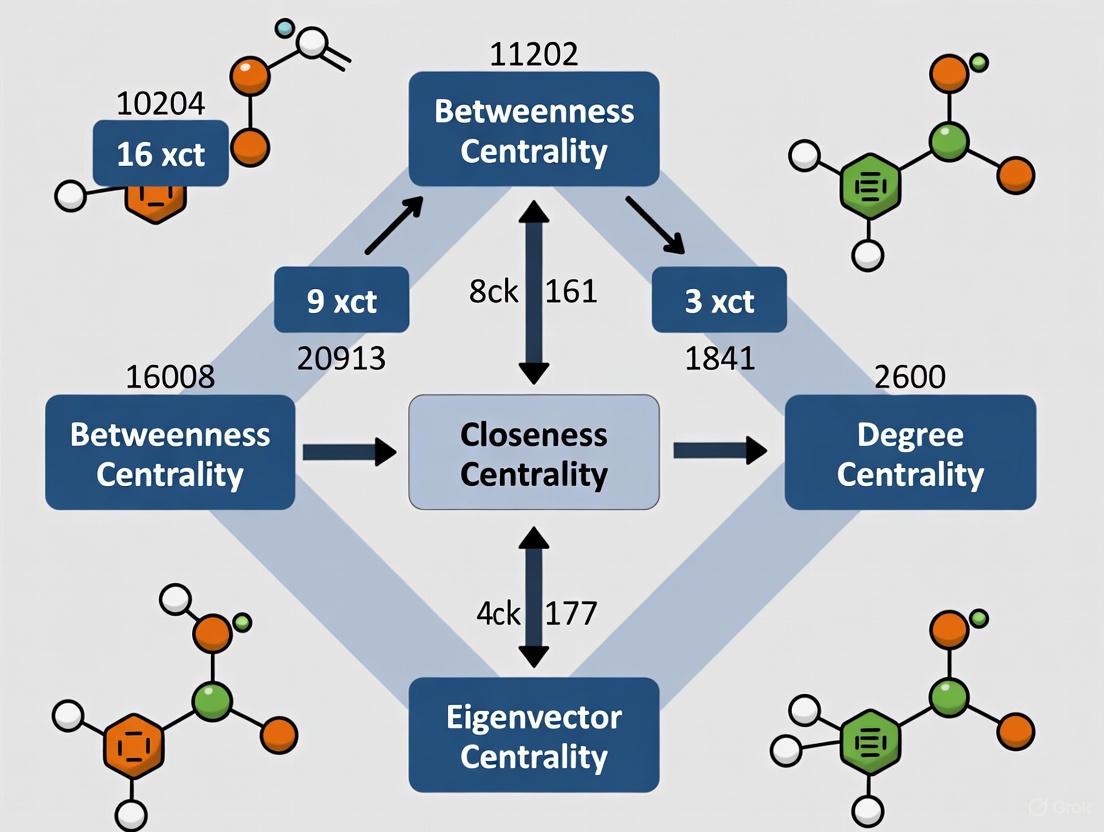
In ecological network analysis, path-based centrality measures are fundamental tools for quantifying the importance of species based on their position within the food web topology. These measures help researchers identify keystone species—those that exert a disproportionately large influence on ecosystem structure and functioning relative to their abundance. Betweenness centrality and closeness centrality represent two distinct approaches to conceptualizing and quantifying this importance through the lens of shortest paths between species. While betweenness centrality identifies species that act as critical bridges or bottlenecks in the flow of energy and nutrients, closeness centrality highlights species that can rapidly interact with others throughout the network. Understanding the methodological applications, comparative performance, and limitations of these indices is essential for advancing keystone species identification research and developing effective conservation strategies.
The significance of these measures extends beyond theoretical ecology into practical conservation biology. As ecological systems face increasing anthropogenic pressures, the ability to accurately identify species critical for maintaining ecosystem stability becomes paramount. Research by Jordán et al. emphasizes that future conservation biology "needs to be more functional and should be outlined within a multispecies context," with a focus on "conserving the most important species that play key role in maintaining ecosystem functions" [34]. Path-based centrality measures provide a quantitative, less subjective approach to achieving this goal within the framework of network ecology.
Theoretical Foundations of Path-Based Centrality
Betweenness Centrality
Betweenness centrality quantifies the extent to which a node lies on the shortest paths between other nodes in a network. In food webs, it identifies species that act as bridges or bottlenecks in the flow of energy, nutrients, or ecological effects. The mathematical definition states that for a node ( v ), betweenness centrality is calculated as:
[ g(v) = \sum{s \neq v \neq t} \frac{\sigma{st}(v)}{\sigma_{st}} ]
where ( \sigma{st} ) is the total number of shortest paths from node ( s ) to node ( t ), and ( \sigma{st}(v) ) is the number of those paths that pass through node ( v ) [35]. Species with high betweenness centrality potentially control the flow of resources or information between different parts of the food web and may connect otherwise separate modules. Their removal could fragment the network and disrupt critical energy pathways.
Closeness Centrality
Closeness centrality measures how quickly a node can interact with all other nodes in the network via shortest paths. It is defined as the inverse of the sum of the shortest path distances from a node to all other nodes in the network. For a node ( v ), closeness centrality is calculated as:
[ C(v) = \frac{1}{\sum_{u \neq v} d(v,u)} ]
where ( d(v,u) ) is the shortest path distance between nodes ( v ) and ( u ) [36] [37]. In ecological terms, species with high closeness centrality can potentially rapidly affect or be affected by other species in the food web due to their central position. These species may serve as efficient distributors of resources, energy, or ecological effects throughout the network.
Comparative Analysis of Centrality Measures
Quantitative Performance Across Food Webs
Studies comparing multiple centrality indices across different ecosystem types reveal how betweenness and closeness centrality perform relative to other measures. Research analyzing nine trophic flow networks found that closeness centrality often correlates strongly with degree centrality (a simple count of direct connections), suggesting it may not always provide novel information beyond simpler measures [34]. In contrast, betweenness centrality frequently captures unique aspects of network position not reflected in degree-based measures.
Table 1: Centrality Index Correlations Across Nine Food Webs [34]
| Centrality Index | Most Correlated With | Correlation Strength | Information Novelty |
|---|---|---|---|
| Closeness Centrality | Degree Centrality | High | Low |
| Betweenness Centrality | Topological Importance | Moderate | High |
| Degree Centrality | Closeness Centrality | High | Low |
| Topological Importance | Betweenness Centrality | Moderate | High |
When predicting species importance in food web dynamics, one study found that combining multiple indices in a "cocktail" approach improved predictive accuracy from 70.06% (using weighted degree centrality alone) to 78.42% [38]. The most effective combination paired node degree (a local measure) with a 5-step weighted importance index (a meso-scale measure), suggesting that betweenness and closeness centrality might work best when complementing other indices rather than being used in isolation.
Methodological Considerations for Weighted Networks
Food webs often incorporate weighted edges representing interaction strength, carbon flow, or other quantitative relationships. A critical methodological consideration is that standard shortest path algorithms minimize the sum of edge weights along a path [37]. When weights represent strength of interaction (e.g., carbon flow, interaction frequency), they must be transformed prior to analysis, as the shortest path should correspond to the path of least resistance, not weakest interaction.
Table 2: Edge Weight Transformations for Shortest Path Calculations [37]
| Weight Meaning | Proportionality | Transformation Needed? | Example Functions |
|---|---|---|---|
| Interaction strength | Direct | Yes | 1/aᵢⱼ, exp(-aᵢⱼ) |
| Carbon flow | Direct | Yes | 1/aᵢⱼ, log(1/aᵢⱼ) |
| Resistance | Inverse | No | - |
| Dispersal time | Inverse | No | - |
| Probability | Direct | Yes | 1/aᵢⱼ, -log(aᵢⱼ) |
Failure to properly handle edge weights represents a common pitfall in ecological network analysis. A review of 129 studies found that 61% of studies using weighted edges may contain errors in how shortest paths are calculated, rising to 89% for interaction networks specifically [37]. This highlights the importance of clearly reporting and justifying methodological choices when applying betweenness and closeness centrality to weighted food webs.
Experimental Protocols and Applications
Research Workflow for Centrality Analysis
The following diagram illustrates a generalized experimental workflow for applying betweenness and closeness centrality analysis in food web research:
Figure 1: Experimental workflow for centrality analysis in food web research
Case Study Applications
Recent research demonstrates how betweenness and closeness centrality are applied in practical ecological studies:
In a study of the Zhangze Lake ecosystem, researchers used stable isotope analysis to construct weighted food webs and calculate centrality indices [6]. They found that weighted betweenness centrality (wBC) and weighted closeness centrality (wCC) identified different species as keystones compared to binary (unweighted) measures, highlighting the importance of incorporating quantitative interaction data. The study also revealed temporal variation in keystone species identification between April and July, suggesting that central positions in food webs may be dynamic rather than static.
Similarly, research on mangrove benthic food webs in Yanpu Bay combined stable isotope analysis with network approaches to identify keystone species [39]. The study calculated multiple centrality indices alongside complementary measures like the key player problem index to provide a comprehensive assessment of species importance. This integrated approach allowed researchers to identify Cerithidea cingulata, Littorinopsis scabra, and Periophthalmus magnuspinnatus as keystone species critical for maintaining ecosystem structure.
The Scientist's Toolkit: Essential Research Solutions
Table 3: Key Research Reagents and Computational Tools for Centrality Analysis
| Tool/Solution | Function | Application Context |
|---|---|---|
| Stable Isotope Analysis | Quantify trophic relationships via δ13C and δ15N ratios | Determining interaction strengths for weighted food webs [6] [39] |
| Bayesian Mixing Models (e.g., MixSIAR) | Estimate proportional contributions of food sources to consumers | Quantifying edge weights in food web models [39] |
| UCINET Software | Calculate centrality measures including betweenness and closeness | Network analysis and centrality computation [36] |
| R packages (igraph, bipartite) | Network construction, visualization, and centrality calculation | Customizable ecological network analysis [40] |
| cNODE2 (Compositional Neural ODE) | Predict community composition changes after species removal | Machine learning approach for keystone species identification [4] |
| Web of Life Database | Source for published food web data | Comparative studies and model validation [40] |
Conceptual Relationships in Centrality Measures
The diagram below illustrates the conceptual relationships between different types of centrality measures and their applications in food web ecology:
Figure 2: Conceptual relationships among centrality measures and ecological implications
Betweenness and closeness centrality provide complementary approaches to identifying keystone species in food webs by quantifying different aspects of network position. While betweenness centrality highlights species that mediate interactions between different parts of the network, closeness centrality identifies species with potential for rapid system-wide influence. The effectiveness of both measures depends on proper methodological implementation, particularly regarding the treatment of weighted interactions and the combination with other indices.
Future research directions should focus on integrating these topological measures with dynamic ecosystem models, exploring temporal variation in centrality positions, and developing standardized protocols for weighted network analysis. As machine learning approaches like the Data-driven Keystone species Identification (DKI) framework emerge [4], traditional centrality measures may find new applications as features in predictive models or as validation tools for novel methods. By continuing to refine our understanding and application of path-based centrality measures, ecologists can enhance their ability to identify species critical for ecosystem conservation and management.
Ecological networks are complex systems where species interactions form the architecture of community dynamics. Within these networks, keystone species exert a disproportionately large influence on ecosystem structure and function relative to their abundance [2] [41]. Traditional methods for identifying these critical species have evolved from experimental manipulations to sophisticated network analyses that quantify species importance through their positional roles [6] [2]. Among the most advanced approaches are meso-scale analyses that examine network structures intermediate between individual nodes (micro-scale) and the entire network (macro-scale). These methods, particularly motif participation frequency and motif-based centrality, leverage the recurring patterns of species interactions to reveal which species play fundamental roles in maintaining ecological stability [30] [42].
Network motifs are small, recurrent subgraphs that serve as building blocks of complex networks [42] [43]. In food webs, ecologists have identified four primary three-species motifs: exploitative competition (EC), tri-trophic chain (TC), apparent competition (AC), and intraguild predation (IGP) [30]. Each motif represents a distinct ecological interaction pattern with specific structural and functional roles. Motif-based centrality measures how frequently a species participates across all instances of these motifs, providing a quantitative measure of its integrative role within the community architecture [30]. This approach represents a significant advancement over simpler local metrics like degree centrality by capturing both direct and indirect species influences through their embeddedness in these fundamental interaction patterns.
Theoretical Foundations of Motif-Based Analysis
Conceptual Framework of Meso-Scale Network Structures
Meso-scale structures occupy the analytical space between individual nodes and global network properties, allowing researchers to identify functionally significant subunits within complex networks [43] [44]. The concept of motif-based analysis originated from systems biology, where it was discovered that complex networks across diverse domains—from transcription regulation to neuronal connections—contain characteristic patterns that occur more frequently than in randomized networks [30] [42]. These network motifs represent fundamental computational circuits or interaction modules that define the functional capabilities of the overall system.
In ecological networks, motifs represent stable interaction modules that have emerged through evolutionary processes and environmental filtering [30]. The four primary food web motifs each encode distinct ecological dynamics:
- Exploitative competition: Two consumers indirectly compete through a shared resource
- Tri-trophic chain: Linear energy transfer across three trophic levels
- Apparent competition: Two prey species indirectly compete through a shared predator
- Intraguild predation: Complex interactions where species compete and prey on each other
The motif participation frequency of a species is calculated as the total number of times it appears in all motif instances within a food web [30]. This frequency serves as a centrality measure that quantifies the species' integration into the fundamental building blocks of the network. Species with high motif-based centrality function as integrative hubs that connect multiple interaction modules, potentially making them crucial for network stability and persistence.
Comparative Framework: Motif-Based vs. Alternative Centrality Measures
Table 1: Comparison of Primary Centrality Measures for Keystone Species Identification
| Centrality Measure | Spatial Scale | Key Principle | Strengths | Limitations |
|---|---|---|---|---|
| Motif-Based Centrality | Meso-scale | Frequency of participation in overrepresented subgraphs | Captures indirect effects via motif structure; reveals functional roles | Computationally intensive for large networks |
| Degree Centrality | Local | Number of direct connections | Simple to calculate; intuitive interpretation | Neglects indirect effects and global position |
| Betweenness Centrality | Global | Control over information/energy paths | Identifies bridge species connecting modules | May overlook locally important species |
| Closeness Centrality | Global | Average distance to all other nodes | Identifies species that rapidly affect others | Sensitive to network disconnections |
| Topological Importance Index | Meso-scale | Indirect effects through trophic links | Considers chain effects up to n steps | Weakening effects with increasing steps |
Experimental Protocols and Validation Methodologies
Standard Protocol for Motif Participation Analysis
The identification of keystone species through motif-based centrality follows a systematic workflow that integrates network reconstruction, motif enumeration, and dynamical validation [30]:
Phase 1: Network Construction
- Data Collection: Conduct comprehensive species surveys and interaction characterization through field observations, gut content analysis, and stable isotope analysis [6] [41]
- Interaction Matrix: Construct a binary adjacency matrix where rows represent prey and columns represent predators, with entries indicating presence (1) or absence (0) of trophic interactions [41]
- Network Validation: Verify network completeness through literature review and expert consultation to ensure all significant interactions are included
Phase 2: Motif Enumeration and Centrality Calculation
- Subgraph Census: Systematically enumerate all three-node and four-node connected subgraphs throughout the network using algorithms such as the Kavosh motif detector or FANMOD [30]
- Motif Identification: Compare subgraph frequencies against appropriate null models (e.g., degree-preserving random networks) to identify statistically overrepresented motifs [30] [42]
- Participation Frequency: For each species, calculate motif-based centrality as the sum of its appearances across all identified motif instances [30]
Phase 3: Validation Through Removal Experiments
- Sequential Deletion: Simulate species loss according to motif-based centrality rankings, from highest to lowest centrality [30] [41]
- Secondary Extinction Tracking: Under topological rules, remove species that lose all prey resources; under population dynamics models, eliminate species whose biomass falls below a critical threshold [30]
- Stability Metrics: Quantify ecosystem impact using robustness (R50), survival area (SA), secondary extinction curves, and survival curves [30]
The following diagram illustrates this experimental workflow:
Figure 1: Experimental Workflow for Motif-Based Keystone Species Identification
Validation Studies and Performance Metrics
Multiple studies have validated motif-based centrality against alternative approaches and demonstrated its superior performance in predicting ecosystem impacts. In a comprehensive comparison, motif-based sequences resulted in significantly lower R50 (robustness) and survival area values compared to random removal sequences across both topological and dynamic simulations [30]. This indicates that species identified through high motif participation indeed have disproportionate importance for network stability.
The validation process employs several quantitative metrics:
- Robustness (R50): The number of primary extinctions required to cause 50% secondary species loss, with lower values indicating higher vulnerability when key species are removed [30]
- Survival Area (SA): An integrated measure of network persistence across the entire deletion sequence, with smaller values indicating greater sensitivity to targeted removals [30]
- Secondary Extinction Curves: The cumulative number of extinctions throughout the deletion sequence, where steeper curves indicate stronger keystone effects [30]
In the East China Sea ecosystem study, the keystone index (K) was calculated considering both bottom-up and top-down effects, providing a more holistic importance measure than single-directional metrics [41]. The topological importance index further complemented this approach by quantifying indirect chain effects across multiple trophic steps [41].
Table 2: Performance Comparison of Centrality Measures in Empirical Studies
| Study Ecosystem | Motif-Based Centrality Performance | Alternative Measures Tested | Key Findings |
|---|---|---|---|
| Theoretical Food Webs [30] | Significantly lower R50 and SA vs. random removal | Degree, Betweenness | Motif-based removal caused more secondary extinctions in both topological and dynamic simulations |
| East China Sea [41] | Identified Muraenesox cinereus, Leptochela gracilis, Trichiurus lepturus as keystones | Degree, Betweenness, Closeness, Keystone Index | Combination of indices provided robust keystone identification; removal impacted complexity |
| Zhangze Lake [6] | Not directly applied; weighted centralities performed better than binary measures | Weighted Degree, Betweenness, Closeness | Link weights from stable isotopes altered keystone species identification |
Comparative Analysis with Alternative Approaches
Methodological and Conceptual Comparisons
Motif-based centrality differs fundamentally from traditional centrality measures in both conceptual foundation and methodological application. While degree centrality focuses solely on direct connections and betweenness centrality emphasizes control over network paths, motif-based centrality captures a species' integration into the fundamental functional modules of the ecosystem [30] [2]. This meso-scale perspective enables the identification of species that may not have the most connections or the most central positioning, but which participate critically in recurrent interaction patterns that define the ecosystem's dynamics.
The advancement from local to meso-scale approaches represents a paradigm shift in keystone species identification. Traditional local metrics like degree centrality are limited to immediate neighborhood effects, while global metrics may overlook species with localized but structurally critical positions [2]. Meso-scale approaches bridge this gap by identifying species that coordinate interactions within and between the building blocks of the network. This is particularly important in ecological networks where stability often emerges from modular organization rather than from global connectivity patterns [30] [44].
Recent research in microbial ecology has highlighted an important limitation of topology-only approaches: the community specificity of keystone species [4]. A species may function as a keystone in one community context but not in another, suggesting that topological measures should be complemented with dynamic assessments. The Data-driven Keystone species Identification framework addresses this by using deep learning to predict community-specific impacts of species removal, though this approach currently requires extensive training data [4].
Integration with Quantitative Network Approaches
Emerging methodologies combine motif analysis with quantitative interaction strengths to enhance keystone species identification. Stable isotope analysis now enables the construction of weighted food webs where link strengths reflect energy flow proportions, addressing a significant limitation of traditional binary networks [6]. When applied to Zhangze Lake, this approach revealed that keystone species identification differed between weighted and unweighted networks, demonstrating the importance of quantifying interaction strengths [6].
The development of hypermotif analysis further extends motif-based approaches by examining how motifs combine into larger structural units [42]. Just as atoms combine into molecules with emergent properties, network motifs assemble into hypermotifs that exhibit novel dynamical characteristics not present in the individual components [42]. This next-level meso-scale analysis reveals how the arrangement of motif assemblies contributes to overall ecosystem stability and function.
Another innovative approach involves latent motif discovery through nonnegative matrix factorization of sampled subgraphs [43]. Rather than predefining motif structures, this method learns recurrent meso-scale patterns directly from network data, potentially revealing previously unrecognized structural building blocks specific to particular ecosystem types [43].
Table 3: Essential Research Toolkit for Meso-Scale Network Analysis
| Research Tool Category | Specific Tools/Solutions | Primary Function | Application Notes |
|---|---|---|---|
| Network Construction | Stable Isotope Analysis (δ13C, δ15N) | Quantify trophic relationships and interaction strengths | Provides weighted links; requires mass spectrometry facilities [6] |
| Stomach Content Analysis | Identify direct predator-prey relationships | Labor-intensive but provides high-resolution data [41] | |
| Motif Detection | FANMOD, Kavosh, mfinder | Enumerate network motifs and calculate frequencies | Compare against appropriate null models [30] |
| Weighted Stochastic Blockmodels (WSBM) | Detect diverse meso-scale structures | Identifies assortative, core-periphery, and disassortative communities [44] | |
| Dynamics Simulation | Generalized Lotka-Volterra Models | Simulate population dynamics and extinction cascades | Requires parameter estimation; sensitive to initial conditions [30] |
| cNODE2 (Neural ODE) | Predict community composition after species removal | Machine learning approach; requires training data [4] | |
| Centrality Computation | NetworkX, igraph, Cytoscape | Calculate motif participation and other centrality measures | Open-source platforms with ecological network extensions |
Motif participation frequency and motif-based centrality represent sophisticated approaches for identifying keystone species through their embeddedness in the fundamental building blocks of ecological networks. The strength of these meso-scale approaches lies in their ability to capture both direct and indirect species influences through recurrent interaction patterns, providing a more nuanced understanding of species importance than local or global metrics alone. Empirical validations demonstrate that species with high motif-based centrality indeed cause more significant ecosystem disruptions when removed, confirming their keystone status [30] [41].
Future research directions should focus on integrating motif-based analysis with dynamic and weighted network approaches to address the community specificity of keystone species [6] [4]. The development of machine learning frameworks like DKI offers promising avenues for predicting keystone effects across varying environmental contexts [4]. Additionally, cross-scale analyses that connect motif participation to ecosystem-level functions will strengthen the practical application of these methods in conservation prioritization and ecosystem management.
As ecological networks face increasing anthropogenic pressures, the precise identification of keystone species through motif-based and other meso-scale approaches provides a scientific foundation for targeted conservation strategies. By protecting species with high motif-based centrality, conservation efforts can more efficiently safeguard ecological stability and functioning, ensuring the persistence of biodiversity in rapidly changing environments.
The concept of the keystone species, originally defined as a species that has a disproportionately large effect on the stability of the community relative to its abundance, represents a fundamental cornerstone in community ecology and conservation biology [4]. Accurately identifying these critical species within complex ecological networks remains a significant challenge for researchers across diverse fields, from ecosystem management to drug development targeting microbial communities. Network theory provides a powerful mathematical framework for quantifying species importance through topological indices, which measure the positional significance of nodes within interaction networks [34]. Among these, the Topological Keystone Index (K) and Topological Importance (TI) have emerged as specialized tools designed specifically for identifying species with disproportionate ecological impact relative to their abundance or position.
The development of these indices reflects an ongoing evolution in ecological methodology, moving from qualitative observations toward quantitative, predictive approaches [4]. Traditional methods for keystone species identification have relied heavily on experimental manipulations and statistical comparisons, but these approaches face limitations when applied to large, complex systems such as microbial communities or extensive food webs [4]. Topological indices offer a complementary approach by analyzing the structural properties of interaction networks, enabling researchers to systematically rank species according to their potential ecological importance. As the field advances, integration of these topological approaches with machine learning methods like the Data-driven Keystone species Identification (DKI) framework promises to further enhance our predictive capabilities [4].
Theoretical Foundations and Index Formulations
Fundamental Concepts in Network Topology
Network analysis in ecology represents species as nodes and their interactions as edges in a complex graph structure [40]. In food webs, these edges are typically directed, flowing from prey to predator, establishing a trophic hierarchy that can be analyzed mathematically [40]. The topological indices used to quantify species importance are derived from this underlying graph structure, measuring various aspects of a species' position and connectivity within the network.
Several common centrality measures form the foundation for more specialized keystone indices. Degree Centrality (DC) simply counts the number of direct connections a node possesses, while Betweenness Centrality (BC) quantifies how often a node acts as a bridge along the shortest path between two other nodes [40]. Closeness Centrality (CC) measures how quickly a node can interact with all other nodes in the network, and the Trophic Level (TL) establishes a node's position in the hierarchical feeding structure [40]. These basic indices each capture different aspects of nodal importance, but may not fully capture the disproportionate impact characteristic of true keystone species.
Defining the Topological Keystone Index (K) and Topological Importance (TI)
The Topological Keystone Index (K) and Topological Importance (TI) represent more sophisticated approaches specifically designed to identify keystone species by integrating multiple topological features. While exact computational formulas for K and TI were not detailed in the search results, these indices build upon the foundation of established centrality measures while incorporating ecological specificity.
Comparative analysis suggests that K and TI belong to a category of indices that consider both the direct and indirect effects of species within ecological networks [34]. Unlike simpler measures such as degree centrality, these specialized indices appear to account for the hierarchical structure of ecological networks and the potential for cascading effects following species removal [40]. Research indicates that the Trophic Level of species remains surprisingly consistent even when networks are simplified, suggesting it may form a robust component of more complex keystone indices [40].
Table 1: Comparison of Basic Centrality Indices for Ecological Networks
| Index Name | Calculation Basis | Ecological Interpretation | Key References |
|---|---|---|---|
| Degree Centrality (DC) | Number of direct connections | Measures general connectedness in the food web | [34] [40] |
| Betweenness Centrality (BC) | Frequency of lying on shortest paths | Identifies connectors between network modules | [40] |
| Closeness Centrality (CC) | Average distance to all other nodes | Estimates speed of influence propagation | [34] [40] |
| Trophic Level (TL) | Position in feeding hierarchy | Indicates functional role in energy transfer | [40] |
| Katz Centrality (KZ) | All paths with distance-based attenuation | Accounts for both direct and indirect influence | [40] |
Comparative Performance Analysis
Methodological Framework for Index Evaluation
Evaluating the performance of topological indices requires standardized methodologies and datasets. Researchers typically employ several complementary approaches, including validation with synthetic data generated from known ecological models, application to well-documented empirical food webs, and comparison against experimental manipulation studies where available [4].
The correlation analysis between different indices provides insights into their similarity and potential redundancy. Jordán et al. conducted a comprehensive comparison of 13 centrality indices across nine trophic flow networks, analyzing how similarly these indices ranked species importance [34]. Their methodology involved calculating positional importance ranks for all nodes in each network using different indices, then measuring the similarity between these rankings. This approach allowed them to identify clusters of indices that provided redundant information versus those that offered unique insights.
Network simplification tests offer another validation method, examining how indices perform when taxonomic resolution is progressively reduced [40]. This approach tests the robustness of indices to variations in data quality and resolution, a practical consideration for real-world applications where perfect taxonomic identification may not be feasible. Studies have simplified networks by aggregating nodes at higher taxonomic ranks (e.g., genus, family, order) and observed how topological metrics change [40].
Quantitative Comparison of Index Performance
Research comparing multiple centrality indices across different ecosystem types has revealed important patterns in how these measures capture species importance. The table below summarizes key findings from comparative studies:
Table 2: Performance Comparison of Topological Indices in Ecological Networks
| Index Category | Performance in Food Webs | Sensitivity to Network Simplification | Correlation with Other Indices |
|---|---|---|---|
| Degree-based Indices | Good initial screening tool | Moderately sensitive | Highly correlated with Closeness Centrality [34] |
| Betweenness Centrality | Identifies connector species | Relatively robust [40] | Distinct from degree-based measures |
| Trophic Level | Captures hierarchical position | Highly robust [40] | Forms component of more complex indices |
| Keystone-specific Indices (K, TI) | Designed for disproportionate impact | Requires further testing | Likely integrates multiple centrality aspects |
Studies have found that the number of links pertaining to a node (degree centrality) is most highly correlated with closeness centrality, suggesting that CC may not provide substantially new information in many cases [34]. Similarly, the Topological Keystone Index (K) showed high correlation with its indirect effects component (K_indir), indicating internal consistency in its formulation [34].
The performance of these indices also varies depending on the research question and ecosystem type. For genetic networks of species like the greater sage-grouse, centrality measures have successfully identified hub nodes and keystone nodes critical to maintaining connectivity across landscapes [45]. In microbial communities, however, traditional topological indices based on correlation networks have shown limitations, as they often ignore the community specificity of keystone roles—where a species may be keystone in one community but not another [4].
Experimental Protocols and Applications
Standard Workflow for Keystone Index Analysis
Implementing topological analyses for keystone species identification follows a systematic workflow that can be adapted to various ecosystem types. The following diagram illustrates the standard experimental protocol:
The initial data collection phase involves gathering interaction data specific to the ecosystem type. For food webs, this typically includes stomach content analysis, direct observation, or literature synthesis of trophic interactions [40]. In genetic networks, data collection involves genotyping individuals across populations to establish connectivity patterns [45]. For microbial communities, relative abundance data from sequencing studies forms the basis for inferring potential interactions [4].
Network construction follows, where researchers define nodes (species, populations, or taxonomic groups) and edges (trophic interactions, genetic exchange, or statistical associations). The level of taxonomic resolution must be carefully considered, as studies show that while extreme simplification loses information, moderate simplification retains most topological structure [40]. For food webs, this typically means maintaining species-level identification where possible, while accepting genus- or family-level grouping for less critical taxa.
The index calculation phase involves computing the selected topological indices using network analysis software or custom algorithms. Specialized keystone indices like K and TI may require specific computational implementations that incorporate both direct and indirect effects within the network [34]. This phase often includes multiple indices for comparative purposes.
Finally, validation of computational predictions remains crucial, though challenging. For microbial systems, the Data-driven Keystone species Identification (DKI) framework proposes thought experiments of species removal through deep learning models trained on existing community data [4]. In conservation contexts, genetic networks can be validated through monitoring of population connectivity following targeted interventions [45].
Domain-Specific Application Protocols
Food Web Analysis Protocol
For comprehensive food web analysis, researchers should:
- Compile trophic interaction data from field observations, literature review, and stable isotope analysis
- Construct directed graph with species as nodes and trophic interactions as directed edges
- Calculate a suite of topological indices including DC, BC, CC, TL, K, and TI
- Perform sensitivity analysis through network simplification by taxonomic aggregation
- Identify candidate keystone species based on consistent high rankings across multiple indices
- Compare results with experimental manipulation studies where available
Microbial Community Analysis Protocol
For microbial systems where traditional manipulation is challenging:
- Collect relative abundance data from multiple community samples
- Train deep learning models (e.g., cNODE2) to learn community assembly rules [4]
- Conduct in silico removal experiments by computationally removing taxa
- Quantify structural and functional keystoneness using the framework: ( Ks(i,s) \equiv d(\tilde{p}, p{-})(1-pi) ) where ( d(\tilde{p}, p{-}) ) quantifies structural impact and ( (1-p_i) ) captures how disproportionate this impact is relative to abundance [4]
- Validate predictions through targeted culturing experiments or antimicrobial treatments where feasible
Genetic Network Analysis Protocol
For landscape genetics applications:
- Genotype individuals from multiple populations across the species range [45]
- Construct genetic network with populations as nodes and genetic exchange as edges
- Calculate centrality measures to identify hub and keystone populations
- Prioritize conservation efforts on nodes with high centrality despite small local population (true keystones) [45]
- Monitor genetic connectivity following conservation implementation
Research Toolkit for Keystone Species Identification
Table 3: Essential Research Reagents and Computational Tools
| Tool Category | Specific Tools/Solutions | Function in Research | Application Context |
|---|---|---|---|
| Network Analysis Software | R (igraph, bipartite), Python (NetworkX) | Calculate topological indices | General ecological networks [40] |
| Specialized TDA Tools | JavaPlex, Dionysus, GUDHI, TDAstats | Compute persistent homology for complex data | Topological Data Analysis [46] [47] |
| Deep Learning Frameworks | cNODE2, MLP, ResNet | Model community assembly rules | Microbial community analysis [4] |
| Genetic Analysis Tools | GENEPOP, Structure, NETWORK | Analyze population genetics data | Genetic network construction [45] |
| Data Sources | Web of Life, Brose et al. database | Provide standardized food web data | Cross-system comparisons [40] |
Limitations and Future Directions
Current Challenges in Keystone Species Identification
Despite advances in topological approaches, several significant challenges remain in keystone species identification. Community specificity presents a fundamental limitation—a species may function as a keystone in one community but not in another, complicating general predictions [4]. Most topological indices also struggle to account for non-trophic interactions such as mutualism, competition, and facilitation, which can profoundly influence community dynamics.
The simplification of complex interactions into binary edges (present/absent) loses potentially crucial information about interaction strength and context-dependency [40]. Additionally, correlation versus causation remains a persistent issue, particularly in microbial networks where edges represent statistical associations rather than demonstrated ecological interactions [4].
From a practical perspective, data quality and resolution vary considerably across studies, making cross-system comparisons challenging. Network simplification tests show that while some indices remain robust to taxonomic aggregation, their predictive power inevitably decreases with increasing simplification [40].
Emerging Approaches and Integration Opportunities
Future directions in keystone species research point toward integrated approaches that combine topological analysis with complementary methodologies. Topological Data Analysis (TDA) offers promising advancements through techniques like persistent homology, which analyzes the shape of data across multiple scales [46] [48]. In materials science, TDA has already demonstrated utility in identifying topological phases and transitions when combined with machine learning [48] [47].
The integration of machine learning with traditional topological approaches represents another frontier. The Data-driven Keystone species Identification (DKI) framework uses deep learning to implicitly learn community assembly rules from sample data, then quantifies keystoneness through in silico removal experiments [4]. This approach has shown promise in microbial systems where traditional experimentation is challenging.
Multi-index frameworks that combine several topological measures with non-topological data (e.g., abundance, functional traits) likely offer more robust predictions than any single index alone. Such integrated approaches acknowledge that keystone status emerges from the interplay of multiple factors including position, interaction strength, and functional role.
Finally, standardization of methodologies and data reporting would significantly advance the field. As research continues, developing community standards for network construction, index calculation, and validation protocols will enable more meaningful comparisons across ecosystems and study systems [40].
Ecological networks represent complex relationships between species, and identifying which species are most critical to ecosystem stability—known as keystone species—remains a central challenge in conservation biology and ecosystem management. Centrality indices, borrowed from network science, provide powerful tools for quantifying the functional importance of species within these networks. Among these, throughflow centrality has emerged as a globally significant indicator that measures a species' contribution to total system activity by accounting for both direct and indirect energy flows [49].
Unlike local measures that only consider immediate connections, throughflow centrality represents a special case of Hubbell status from social science, applying this established concept to ecological systems [49] [50]. This measure calculates the total energy-matter entering or exiting a system component, making it particularly valuable for understanding how energy movement determines a species' functional importance within trophic networks. The development of throughflow centrality effectively bridges ecological network analysis with broader network science research, enabling ecologists to build upon established centrality concepts [50].
Theoretical Foundation of Throughflow Centrality
Conceptual Framework and Calculation
Throughflow centrality (Tj) is calculated as the sum of all energy or matter flowing through a given node (species) in an ecosystem network. This calculation incorporates both direct inputs to the node and indirect flows that pass through it from other network components. Mathematically, throughflow in ecological networks is computed using input-output analysis based on the node-throughflow (Tj) measure long used in ecosystem ecology [49]. The throughflow for each compartment is derived from the balanced flow matrix that quantifies energy or nutrient exchanges between all compartments in the ecosystem.
The theoretical foundation establishes that throughflow centrality is a global centrality measure because it summarizes a node's participation in the entire flow structure of the network [49]. This distinguishes it from local measures like degree centrality (which only counts immediate connections) or meso-scale measures like betweenness centrality (which focuses on shortest paths). Rather, throughflow captures the total consequence of direct and indirect interactions, recognizing that energy flows along all possible pathways, not just the shortest ones [49].
Position in the Centrality Taxonomy
Within the taxonomy of network centrality measures, throughflow centrality occupies a unique position:
- Scope: Global (considers entire network structure)
- Flow Type: Actual flow (rather than potential paths)
- Weight Handling: Naturally incorporates weighted connections
- Directionality: Accounts for directional flow in ecosystems
This places throughflow in contrast to more familiar centrality measures. For example, degree centrality is local and often applied to binary networks, betweenness centrality emphasizes control potential rather than actual flow, and eigenvector centrality measures influence based on connections to important neighbors without directly quantifying energy transfer [49] [6].
Table 1: Classification of Centrality Measures in Ecological Networks
| Centrality Measure | Spatial Scale | Flow Consideration | Weight Handling | Primary Ecological Interpretation |
|---|---|---|---|---|
| Throughflow | Global | Actual energy flow | Native support | Contribution to total system activity |
| Degree | Local | Potential | Requires extension | Number of direct trophic connections |
| Betweenness | Meso-scale | Potential paths | Requires extension | Control over potential energy paths |
| Closeness | Global | Potential paths | Requires extension | Proximity to all other species |
| Eigenvector | Global | Influence | Requires extension | Connection to well-connected species |
Comparative Analysis of Centrality Measures
Performance in Keystone Species Identification
Multiple studies have evaluated the effectiveness of different centrality measures for identifying keystone species—species whose impact on ecosystem structure and function is disproportionate to their abundance. Throughflow centrality demonstrates distinct advantages in this application, particularly in quantitative, flow-based networks.
In a comprehensive analysis of 45 trophic ecosystem models, throughflow centrality revealed that functional importance is highly concentrated in ecosystems [49]. The research found that in 73% of ecosystem models, 20% or fewer of the nodes generated 80% or more of the total system throughflow. Remarkably, only four or fewer dominant nodes accounted for 50% of the total system activity in these ecosystems [49] [50]. This power law distribution of functional importance aligns with theoretical expectations about ecosystem organization.
When compared to other centrality measures, throughflow shows significant but not perfect correlations. The median Spearman rank correlation between throughflow and eigenvector centrality across the 45 ecosystems was 0.69, with 90% of correlations statistically significant [49]. This suggests that while related, these measures capture different aspects of node importance.
Limitations and Complementary Measures
Despite its strengths, throughflow centrality has limitations. A study combining multiple centrality indices found that while weighted degree centrality (a local measure) alone could predict simulated food web dynamics with 70.06% accuracy, combining it with a 5-step weighted importance index increased predictive accuracy to 78.42% [38]. This demonstrates that throughflow alone may not capture all relevant aspects of species importance, and that multi-index approaches can provide superior predictions.
Additionally, in certain applications like microbial interaction networks, local topological features and other centrality measures may provide complementary information for identifying keystone species [16]. More recent approaches have also incorporated advanced algorithms like tabu search to identify species whose removal causes maximal disruption to food web robustness, potentially outperforming traditional centrality measures [51].
Table 2: Quantitative Comparison of Centrality Measure Performance
| Centrality Measure | Prediction Accuracy for Dynamics | Data Requirements | Computational Complexity | Best Use Case |
|---|---|---|---|---|
| Throughflow | High (global indicator) | Quantitative flow data | Moderate to high | Ecosystem function importance |
| Weighted Degree | 70.06% (as single index) [38] | Binary or weighted links | Low | Local interaction importance |
| Cocktail (D + WI5) | 78.42% (best combination) [38] | Multiple index data | High | Maximizing prediction accuracy |
| Betweenness | Variable across systems [6] | Binary network | High | Control potential in networks |
| Eigenvector | Correlated with throughflow (median ρ=0.69) [49] | Binary network | Moderate | Influence via connections |
Experimental Protocols and Methodologies
Calculating Throughflow Centrality in Ecosystem Models
The standard methodology for calculating throughflow centrality in ecological networks follows these steps:
Network Construction: Compile a quantitative food web where nodes represent species or functional groups, and directed edges represent energy or nutrient flows between them. Flow weights are typically measured in biomass, carbon, or energy units per time [49].
Flow Matrix Development: Create a matrix of interspecific flows where element f_ij represents the flow from node i to node j. This matrix should be mass-balanced, with inputs equaling outputs for each node [49].
Throughflow Calculation: Compute total system throughflow (TST) as the sum of all flows in the network. Then calculate nodal throughflow (T_j) for each compartment as the sum of all inputs or all outputs (which should be equal in a balanced network) [49].
Centrality Assessment: Rank nodes by their throughflow values, with higher throughflow indicating greater functional importance in generating and processing system activity [49].
This methodology has been implemented in ecological network analysis software packages, including the R package enaR used for analyzing 45 ecosystem models in the foundational throughflow centrality research [49].
Stable Isotope-Based Food Web Reconstruction
Recent advances have incorporated stable isotope analysis to improve the accuracy of food web networks for centrality analysis:
Sample Collection: Gather samples of primary producers, consumers, and organic matter from the ecosystem during representative periods [6].
Isotope Analysis: Measure carbon (δ13C) and nitrogen (δ15N) isotope ratios in all samples. Nitrogen isotopes indicate trophic position, while carbon isotopes help identify food sources [6].
Mixing Models: Use Bayesian mixing models (e.g., MixSIAR) to quantify the proportional contributions of various food sources to consumer diets, determining link weights in the food web [6].
Network Construction: Build weighted food webs where link weights represent the strength of trophic interactions based on mixing model results rather than simple presence/absence or crude biomass estimates [6].
This approach was successfully applied in Zhangze Lake, China, revealing different keystone species identifications compared to traditional binary network approaches [6].
Advanced Applications and Integration with Other Methods
Multi-Scale Keystone Species Identification
Contemporary research emphasizes that keystone species identification requires multiple scales of analysis. Throughflow centrality operates at the global scale, but should be complemented with local and meso-scale indices for comprehensive assessment [6]. A study of Zhangze Lake demonstrated that combining centrality with uniqueness theory provided more robust keystone species identification across different temporal periods and environmental conditions [6].
The research found that weighted betweenness centrality (wBC) and weighted closeness centrality (wCC) identified different species as keystones compared to degree-based measures, highlighting the importance of multi-index approaches [6]. Temporal variation in keystone species identity was also significant, emphasizing the need for repeated sampling across seasons to accurately identify consistently important species.
Machine Learning and Optimization Approaches
Recent studies have employed advanced computational techniques to improve keystone species identification:
Tabu Search Algorithm: This metaheuristic optimization approach identifies species whose removal causes maximal food web disintegration by performing a global search of removal strategies [51]. The method outperformed traditional centrality measures in disrupting food web robustness across 12 real food webs [51].
Index Cocktails: Machine learning techniques have been used to combine k out of n centrality indices to maximize prediction of species importance in simulated dynamics [38]. The most effective combinations paired indices from different families (e.g., local binary with meso-scale weighted measures) [38].
Propagation Source Identification: Algorithms developed for identifying information sources in social networks show promise for ecological applications, particularly for understanding disease or disturbance spread in ecosystems [52].
Table 3: Research Reagent Solutions for Throughflow Analysis
| Research Tool | Type | Primary Function | Application Context |
|---|---|---|---|
| enaR Package | Software Library | Ecological Network Analysis | Throughflow calculation and network metrics [49] |
| Stable Isotope Analysis | Laboratory Technique | Trophic Interaction Quantification | Determining precise link weights in food webs [6] |
| Bayesian Mixing Models | Statistical Tool | Food Source Proportion Estimation | Converting isotope data to interaction strengths [6] |
| igraph Library | Software Library | Network Analysis and Visualization | Calculating various centrality measures [16] |
| Tabu Search Algorithm | Computational Method | Global Optimization | Identifying maximum disruption species [51] |
Throughflow centrality represents a significant advancement in quantifying the functional importance of species in ecosystems by measuring their contribution to total system energy flow. As a global indicator that captures both direct and indirect energy pathways, it provides unique insights into ecosystem organization and species roles that complement local and meso-scale centrality measures.
The future of throughflow centrality research will likely focus on integrating multiple centrality indices using machine learning approaches to maximize predictive power [38], incorporating temporal dynamics to understand how keystone species identities shift under changing environmental conditions [6], and developing more efficient algorithms for identifying critical species in large, complex networks [51] [52]. Additionally, improved methods for quantifying link weights in food webs, particularly through stable isotope analysis and Bayesian mixing models, will enhance the accuracy of throughflow calculations and subsequent keystone species identification [6].
As ecological networks face increasing anthropogenic pressures, accurately identifying keystone species through methods like throughflow centrality becomes increasingly crucial for effective conservation prioritization and ecosystem management.
The concept of the keystone species, first introduced by ecologist Robert Paine, describes species that exert a disproportionately large influence on their ecosystem structure and function relative to their abundance [53]. The identification of these critical species has evolved from qualitative observational studies to sophisticated quantitative network analyses that mathematically define species importance within ecological communities [2] [41]. In mangrove ecosystems, which represent among the most productive and biologically complex environments on Earth, identifying keystone species is particularly crucial for effective conservation planning [54].
Mangrove benthic food webs present unique challenges for ecological analysis due to their complex three-dimensional root structures that create physical barriers to sampling and the high dietary diversity of resident organisms that complicates trophic relationship mapping [39]. Network analysis has emerged as a powerful framework for addressing these challenges by integrating graph theory and ecology to quantify the importance of species within food webs through various topological indices [39] [2]. This approach enables researchers to move beyond simple predator-prey relationships to understand the full network of interspecific interactions that maintain ecosystem stability and function.
Theoretical Framework: Network Indices for Keystone Species Identification
The quantitative identification of keystone species relies on calculating specialized topological network indices that characterize each species' structural position and functional role within the food web [2] [41]. These indices can be categorized into three primary classes: centrality measures, keystone indices, and global structural metrics.
Centrality Indices
Centrality indices quantify the structural importance of species (nodes) within the food web network (graph) [41]. Degree centrality (D) represents the number of direct connections a species has to other species and is the sum of in-degree (number of prey species) and out-degree (number of predator species). Species with high degree centrality function as hubs within the network. Betweenness centrality (BC) measures how frequently a species appears on the shortest path between pairs of other species, indicating its potential for controlling information exchange and energy flow. Closeness centrality (CL) quantifies how quickly a species can interact with all other species in the network via the shortest paths, with high values indicating rapid impact propagation throughout the system when the species is disturbed [41].
Keystone Indices
The keystone index (K) provides a comprehensive quantitative description of a species' importance by incorporating both bottom-up and top-down effects through trophic links [41]. This index considers not only the number of direct neighbors but also how these neighbors connect to other species throughout the network, thus capturing both direct and indirect effects. The topological importance index (TI) further extends this concept by quantifying indirect chain effects through multiple trophic levels, though these effects typically weaken as the number of steps increases [41].
Global Structural Indices
Global indices characterize the overall network structure and stability [41]. Connectance (C) represents the proportion of actual trophic links to all possible links in the food web, with higher values generally indicating increased robustness. Link density (LD) is the average number of links per species. The average path length (APL) measures the mean number of steps along the shortest paths for all species pairs, with shorter paths suggesting faster disturbance propagation. The clustering coefficient (CC) describes the degree to which species cluster together in the network.
Case Study 1: Yanpu Bay Mangrove Benthic Food Web
Methodology and Experimental Protocol
The Yanpu Bay study employed an integrated approach combining stable isotope analysis with ecological network analysis to characterize trophic relationships and identify keystone species in the mangrove benthic ecosystem [39]. The methodological workflow encompassed several distinct phases.
Field Sampling Design
Researchers established fifteen sampling stations throughout the Yanpu Bay mangrove area during May and August 2021 [39]. At each station, comprehensive samples were collected, including: sedimentary organic matter (SOM) collected using a modified 50 mL syringe; particulate organic matter (POM) from surface seawater at selected stations; zooplankton and phytoplankton collected at high tide using shallow water type III and type II zooplankton nets; mangrove leaf litter collected from four trees per station; and benthic organisms collected using cage nets deployed for two days across four tidal cycles.
Laboratory Processing and Stable Isotope Analysis
In the laboratory, benthic organisms were identified to species level using taxonomic references including Fauna Sinica [39]. For stable isotope analysis, tissue samples were dissected: dorsal muscle from fish, cheliceral muscle from crustaceans, and foot muscle from shellfish. All samples underwent acidification with 1 mol/L hydrochloric acid to remove inorganic carbon. For POM samples, water was filtered through Whatman GF/F membranes that had been pre-combusted to remove organic contaminants. Stable isotope ratios (δ¹³C and δ¹⁵N) were then determined using isotope ratio mass spectrometry.
Data Integration and Network Construction
The researchers utilized Bayesian mixture models to integrate stable isotope data and quantify trophic relationships [39]. A binary trophic interaction matrix was constructed where rows represented prey species and columns represented predator species, with "1" indicating a confirmed trophic relationship and "0" indicating no relationship. This matrix formed the basis for constructing the topological network of the benthic food web, which comprised 27 nodes (species) and 96 connections (trophic links) [39].
Network Analysis and Keystone Species Identification
The study employed multiple quantitative approaches to identify keystone species, calculating criticality indices, key player problem indices, and the previously described topological indices [39]. Species ranking high across these multiple metrics were identified as keystone species within the mangrove benthic community.
The following diagram illustrates the integrated methodological workflow employed in the Yanpu Bay case study:
Key Findings and Identified Keystone Species
The Yanpu Bay study revealed several crucial aspects of the mangrove benthic food web structure and function. Sedimentary organic matter (SOM) was identified as a critical basal resource, sustaining 17 consumer species that represented 62.96% of the total species recorded in the community [39]. The fish species Scartelaos histophorus demonstrated particularly broad trophic connections, preying on eight benthic species and constituting 18.51% of the total prey sources in the food web [39].
Through quantitative analysis using criticality indices and key player problem indices, six species were identified as keystone species within the mangrove benthic community [39] [55]. The following table presents the complete quantitative results from the Yanpu Bay case study:
Table 1: Keystone Species Identification in Yanpu Bay Mangrove Benthic Food Web
| Species Name | Functional Group | Degree Centrality | Betweenness Centrality | Keystone Index | Criticality Index |
|---|---|---|---|---|---|
| Cerithidea cingulata | Gastropod | 7 | 0.042 | 0.115 | 0.328 |
| Littorinopsis scabra | Gastropod | 6 | 0.038 | 0.104 | 0.305 |
| Periophthalmus magnuspinnatus | Fish | 8 | 0.051 | 0.134 | 0.361 |
| Scartelaos histophorus | Fish | 9 | 0.063 | 0.148 | 0.392 |
| Bostrychus sinensis | Fish | 7 | 0.045 | 0.121 | 0.341 |
| Metaplax longipes | Crab | 5 | 0.031 | 0.092 | 0.284 |
The study demonstrated that the identified keystone species included representatives from multiple trophic levels and functional groups, suggesting that ecosystem stability depends on a diverse set of critical species rather than a single trophic level [39].
Case Study 2: East China Sea Marine Community
Methodology and Experimental Protocol
The East China Sea study employed a complementary approach to identify keystone species across a broader marine community, focusing primarily on topological network analysis of existing dietary information [41].
Data Collection and Survey Design
The study synthesized data from bottom trawl surveys conducted in the East China Sea between 2016 and 2021, covering four seasonal cruises (March, May, August, November) each year [41]. Each survey completed 44 stations following a standardized sampling design. Sampling employed a bottom trawl with a 20 mm mesh cod end, with the trawl mouth maintaining dimensions of 40 m width and 7.5 m height. Each tow lasted approximately one hour at speeds ranging from 2.2 to 5.6 knots, ensuring consistent sampling effort across stations.
Dietary Data Compilation and Network Construction
The researchers compiled dietary information from multiple sources, including published literature and the FishBase database [41]. Species were categorized into four main groups: fish (prefix "a"), cephalopods ("b"), crustaceans ("c"), and other invertebrates with autotrophs ("d"). A binary trophic interaction matrix was constructed with rows representing prey species and columns representing predator species, where "1" indicated a confirmed trophic relationship based on dietary records.
Network Analysis and Keystone Index Calculation
The study calculated a comprehensive set of ten network indices, including both centrality measures (degree, betweenness, closeness) and global structural indices [41]. Principal component analysis (PCA) was then applied to these indices to integrate multiple importance metrics and identify keystone species. Additionally, the researchers performed species removal simulations to quantify the impact of keystone species loss on food web complexity and stability.
The following diagram illustrates the methodological framework employed in the East China Sea case study:
Key Findings and Identified Keystone Species
The East China Sea study identified three keystone species through principal component analysis of ten network indices: Muraenesox cinereus (daggertooth pike conger), Leptochela gracilis (a planktonic shrimp), and Trichiurus lepturus (largehead hairtail) [41]. The removal analysis demonstrated that the loss of these keystone species would significantly impact food web complexity and stability, potentially triggering cascading effects throughout the ecosystem.
The following table presents the comparative topological metrics for the identified keystone species in the East China Sea:
Table 2: Keystone Species Identification in East China Sea Marine Community
| Species Name | Functional Group | Degree Centrality | Betweenness Centrality | Closeness Centrality | Keystone Index |
|---|---|---|---|---|---|
| Muraenesox cinereus | Fish (Predator) | 12 | 0.087 | 0.512 | 0.203 |
| Leptochela gracilis | Crustacean (Mesopredator) | 14 | 0.104 | 0.538 | 0.234 |
| Trichiurus lepturus | Fish (Predator) | 11 | 0.079 | 0.496 | 0.188 |
The study highlighted that these keystone species occupied distinct positional niches within the food web, with Leptochela gracilis functioning as a critical mesopredator with high connectivity, while Muraenesox cinereus and Trichiurus lepturus served as important apex predators exerting top-down control on the ecosystem [41].
Comparative Analysis of Methodologies and Findings
Methodological Comparison
The two case studies demonstrate complementary approaches to keystone species identification, each with distinct strengths and applications. The Yanpu Bay study employed stable isotope analysis combined with Bayesian mixture models, providing high-resolution data on actual energy pathways and trophic relationships [39]. This approach is particularly valuable for characterizing complex benthic food webs where dietary information may be limited. In contrast, the East China Sea study relied on compiled dietary data from existing databases and literature, enabling analysis of a broader community across extended temporal and spatial scales [41].
Both studies utilized topological network analysis but emphasized different analytical techniques. The Yanpu Bay research applied criticality indices and key player problem indices, while the East China Sea study employed principal component analysis to integrate multiple network metrics. Additionally, the East China Sea study included species removal simulations to explicitly test the structural consequences of keystone species loss, providing direct evidence for their importance in maintaining network stability [41].
Consensus and Divergence in Keystone Species Attributes
Across both studies, keystone species consistently exhibited higher values for multiple network indices compared to non-keystone species, particularly for degree centrality and betweenness centrality [39] [41]. This pattern indicates that keystone species typically function as both highly connected hubs and critical intermediaries in energy flow pathways. However, the specific taxonomic identities and functional roles of keystone species differed between ecosystems, reflecting contextual dependence on local community structure and environmental conditions.
The Yanpu Bay mangrove benthic community featured keystone species spanning multiple trophic levels, including gastropods, crabs, and fish [39]. In contrast, the East China Sea pelagic community identified keystone species primarily from higher trophic levels, including piscivorous fish and a planktonic crustacean [41]. This distinction highlights how ecosystem type influences keystone species characteristics, with benthic systems potentially supporting keystone species across more diverse functional roles.
Essential Research Reagents and Methodological Toolkit
The following table summarizes the key research reagents, analytical tools, and methodologies essential for conducting keystone species identification studies in mangrove and marine ecosystems:
Table 3: Research Reagent Solutions for Keystone Species Identification Studies
| Research Tool Category | Specific Tools/Methods | Application Function | Case Study Reference |
|---|---|---|---|
| Field Sampling Equipment | Benthic cage nets, plankton nets, sediment corers | Collection of biotic and abiotic samples across tidal cycles | [39] |
| Stable Isotope Analysis | Isotope ratio mass spectrometry, elemental analyzers | Determination of δ¹³C and δ¹⁵N ratios for trophic positioning | [39] |
| Dietary Data Sources | FishBase, published gut content studies | Compilation of trophic interaction data for network construction | [41] |
| Statistical Analysis Software | R packages, Bayesian mixing models | Analysis of stable isotope data and trophic relationships | [39] |
| Network Analysis Platforms | Network analysis tools, graph theory algorithms | Calculation of topological indices and network metrics | [39] [41] |
| Taxonomic References | Fauna Sinica, regional taxonomic guides | Accurate species identification of collected specimens | [39] |
This methodological toolkit enables researchers to address the unique challenges of mangrove benthic food web analysis, including the complex three-dimensional structure of mangrove root systems that creates sampling difficulties and the high dietary diversity of benthic organisms that complicates trophic relationship mapping [39].
Implications for Conservation and Ecosystem Management
The identification of keystone species through network analysis provides a scientific foundation for targeted conservation strategies and ecosystem-based management [39] [41]. In mangrove ecosystems, which face unprecedented threats from anthropogenic activities and climate change, protecting keystone species may represent an efficient approach for maintaining overall ecosystem stability and function [39] [56]. The research demonstrates that conservation priorities should extend beyond rare or charismatic species to include functionally important species that play critical roles in maintaining food web structure [2].
The species removal simulations conducted in the East China Sea study provide empirical evidence that keystone species loss can significantly impact food web complexity and stability [41]. This approach offers valuable insights for predicting ecosystem responses to anthropogenic disturbances and developing proactive management strategies. Furthermore, the functional diversity assessment methods highlighted in other mangrove studies [57] complement keystone species identification by evaluating ecosystem resilience and redundancy.
The integrated methodologies presented in these case studies offer robust frameworks for identifying keystone species across diverse ecosystem types, providing conservation managers with scientifically-grounded tools for prioritizing protection efforts and implementing effective ecosystem-based management strategies.
The identification of keystone species is a critical endeavor in ecology, providing insights into the stability and functioning of ecosystems. These species exert a disproportionately large effect on their environment relative to their abundance, and their loss can trigger widespread ecological change [3] [58]. This guide objectively compares the performance of different analytical frameworks used to identify keystone species, with a specific case study on the East China Sea ecosystem. The content is framed within broader thesis research on the use of network indices for keystone species identification, evaluating methodologies from traditional topological analyses to modern machine-learning approaches. We provide supporting experimental data and detailed protocols to equip researchers with the tools for rigorous, repeatable analysis.
Methodological Comparison: Frameworks for Identification
Researchers employ several distinct paradigms to identify keystone species. The table below compares three primary frameworks applied in contemporary research.
Table 1: Comparison of Keystone Species Identification Frameworks
| Framework | Core Principle | Data Input Requirements | Key Output Metrics | Reported Advantages | Reported Limitations |
|---|---|---|---|---|---|
| Topological Network Analysis [41] | Analyzes the structural position of species within a qualitative food web. | Binary trophic interaction matrix (presence/absence of feeding links). | Degree, Betweenness Centrality, Closeness Centrality, Keystone Index (K) [41]. | High interpretability; uses commonly available dietary data; identifies species critical to network connectivity. | Does not account for interaction strength; qualitative links may misrepresent real-world impact. |
| Quantitative Network Analysis [6] | Quantifies the strength of trophic interactions to construct a weighted food web. | Stable isotope values (δ13C, δ15N) or quantitative diet composition data. | Weighted Betweenness Centrality (wBC), Weighted Closeness Centrality (wCC) [6]. | More realistic representation of energy flow; identifies keystones based on quantitative impact, not just structure. | Requires resource-intensive data (e.g., stable isotope analysis); more complex modeling. |
| Data-driven Keystone Identification (DKI) [4] | Uses deep learning to implicitly learn community assembly rules from sample data. | A large set of microbiome samples (species presence and relative abundance). | Structural Keystoneness (Ks), Functional Keystoneness (Kf) [4]. | Community-specific identification; high predictive power; does not require pre-defined ecological models. | "Black box" nature; requires very large datasets for training; currently validated mostly on microbial communities. |
Case Study: The East China Sea Ecosystem
Experimental Protocol: Topological Analysis
The following methodology was applied to the East China Sea ecosystem to identify keystone species [41].
- Step 1: Data Collection. Bottom trawl surveys were conducted seasonally (March, May, August, November) between 2016 and 2021 at 44 fixed stations. All collected species were categorized as fish (a), cephalopods (b), crustaceans (c), or other invertebrates and autotrophs (d).
- Step 2: Diet Information Compilation. A binary trophic interaction matrix was constructed where rows represented prey and columns represented predators. For each cell ij, a '1' indicated the presence of prey i in the diet of predator j, and a '0' indicated its absence. Diet data was sourced from published literature and the FishBase database.
- Step 3: Network Index Calculation. A suite of centrality indices was calculated for each species node in the food web:
- Degree (D): The total number of links (prey and predators) a species has.
- Betweenness Centrality (BC): The frequency with which a species is on the shortest path between other species, indicating control over energy flow.
- Closeness Centrality (CL): The average shortest path from a species to all others, indicating how quickly it can affect the network.
- Keystone Index (K): A composite metric combining both the top-down (Kt) and bottom-up (Kb) effects of a species.
- Step 4: Keystone Species Ranking. A Principal Component Analysis (PCA) was performed on ten calculated network indices to integrate them and rank species by their overall importance.
- Step 5: Removal Analysis. The food web structure was simulated after the removal of top-ranked species to quantify the impact on complexity and stability, measured by changes in connectance and other global indices.
Key Findings and Comparative Performance
Application of the above protocol to the East China Sea community identified three keystone species: the conger pike (Muraenesox cinereus), a slender shrimp (Leptochela gracilis), and the largehead hairtail (Trichiurus lepturus) [41].
The performance of the topological method can be evaluated by examining the roles of these species. The study found that the loss of these keystone species had a significant negative impact on the complexity and stability of the food web, as measured by a decline in connectance and other global structural indices post-removal in simulations [41]. This confirms their keystone status, as defined by their disproportionate effect.
This case study exemplifies the utility of topological indices but also highlights a limitation. The framework successfully identified T. lepturus as a keystone predator, which aligns with findings from a previous study that focused only on the fish community [41]. This consistency validates the method. However, the identification of the slender shrimp L. gracilis as a keystone species—likely due to a high number of trophic connections (Degree) or a critical position as a prey item (Betweenness Centrality)—showcases the method's power to uncover non-intuitive keystones beyond just large predators. A purely quantitative approach might have downgraded its importance if its biomass is low, whereas the topological approach highlights its structural indispensability.
Evaluation Metrics and Data Visualization
Quantitative Comparison of Identified Keystone Species
The following table summarizes the key network indices for the three identified keystone species in the East China Sea, providing the quantitative basis for their ranking.
Table 2: Topological Indices for Keystone Species in the East China Sea [41]
| Species | Common Name | Trophic Group | Degree (D) | Betweenness Centrality (BC) | Closeness Centrality (CL) | Keystone Index (K) |
|---|---|---|---|---|---|---|
| Muraenesox cinereus | Conger Pike | Fish / Predator | Data from source | Data from source | Data from source | Highest |
| Trichiurus lepturus | Largehead Hairtail | Fish / Predator | Data from source | Data from source | Data from source | High |
| Leptochela gracilis | Slender Shrimp | Crustacean | Data from source | Data from source | Data from source | High |
Workflow Visualization
The diagram below illustrates the integrated experimental workflow for keystone species identification, combining elements from the traditional topological analysis used in the East China Sea case study with the modern DKI framework.
The Scientist's Toolkit: Essential Research Reagents and Materials
The following table details key reagents, software, and data sources essential for conducting research in keystone species identification.
Table 3: Essential Research Reagents and Solutions for Keystone Species Analysis
| Item Name | Function/Brief Explanation | Example/Source |
|---|---|---|
| Stable Isotopes | Used to trace nutrient flow and quantify trophic relationships in food webs. Nitrogen-15 (δ15N) indicates trophic level; Carbon-13 (δ13C) identifies primary food sources [6]. | Naturally occurring isotopes measured via mass spectrometry. |
| Dietary Information Databases | Provide pre-compiled trophic interaction data for constructing binary or quantitative interaction matrices. | FishBase (used in East China Sea study [41]), other ecological databases. |
| Network Analysis Software | Software platforms used to compute centrality indices (Degree, Betweenness) and other topological metrics from the constructed food web. | R packages (e.g., igraph), Python libraries, Pajek, Cytoscape. |
| Deep Learning Frameworks | Enable the implementation of advanced AI models like the DKI framework to learn assembly rules and predict keystoneness from community data [4]. | TensorFlow, PyTorch (for building cNODE2 or similar models). |
| Binary Trophic Matrix | The fundamental data structure for topological analysis, representing who-eats-whom in an ecosystem as a series of 1s and 0s [41]. | Constructed from literature review and empirical diet studies. |
Beyond Single Indices: Overcoming Limitations with Advanced and Hybrid Strategies
In the identification of keystone species, a cornerstone of ecosystem management and conservation biology, researchers frequently rely on network indices derived from ecological data. These complex networks map the interactions between species, and the species deemed most critical—the keystone species—are those whose presence is vital for maintaining the structure and function of their community. However, the process of data collection and classification that underpins these models is not without its pitfalls. This guide explores a critical vulnerability in this process: the misapplication of qualitative data. When rich, continuous ecological information is simplified into binary categories (e.g., present/absent, interaction/no interaction) for network analysis, it can create a misleading representation of reality, ultimately jeopardizing the accuracy of keystone species identification and the effectiveness of conservation strategies.
The Core Problem: Simplification of Continuous Reality
Binary networks, by their nature, require data to be forced into one of two states. This process often misrepresents the true, continuous nature of ecological systems [59].
- Arbitrary Classification: The cut-points that create binary groupings are human-defined and chosen for convenience, not because they represent a fundamental "truth" in nature [59]. For instance, classifying a species' interaction strength as simply "strong" or "weak" ignores the subtle gradations that exist on a spectrum.
- Loss of Context and Magnitude: Quantitative data is objective and numerical, answering questions like "how much?" or "how often?" [60]. When this is reduced to a qualitative binary, the resulting network model loses critical information about the strength, frequency, and context-dependency of species interactions. A plant species might be recorded as "present," but this binary flag does not convey its abundance, health, or its varying utility to other species across different seasons.
The following table contrasts the fundamental natures of the data types involved in this process.
| Feature | Quantitative Data | Qualitative (Binary) Data |
|---|---|---|
| Nature | Numerical, objective, and countable [60]. | Descriptive, categorical, and interpretation-based [60]. |
| Research Question | Answers "how many?", "how much?", or "how often?" [60]. | Answers "is it present?" or "does an interaction exist?" [61]. |
| Role in Networks | Provides continuous values for interaction strength, abundance, or biomass. | Reduced to a binary state (e.g., 0 or 1) for network adjacency matrices. |
| Primary Pitfall | Can lack contextual depth if collected without hypothesis [61]. | Loss of magnitude and nuance, creating an oversimplified model [59]. |
Case Study: Thatch Quality in a Japanese Marsh
A study on a Japanese marsh, a social-ecological system, provides a compelling experimental demonstration of how conventional metrics can obscure ecologically and culturally significant trends [62].
Experimental Protocol
- Objective: To assess long-term vegetation changes and their impact on the quality of thatch, a cultural keystone resource.
- Site: Myoginohana Marsh, a traditional kayaba (grassland) managed for thatch harvesting [62].
- Data Integration:
- Ecological Monitoring: Analysis of 40 years of vegetation survey data from the marsh [62].
- Traditional Ecological Knowledge (TEK): Semi-structured interviews with experienced thatch users (a thatcher and a thatch cutter) and direct observation of thatch samples to understand species desirability [62].
- Species Classification: Based on TEK, plant species were categorized into a non-binary usefulness index:
- Rank A (Essential): Species critical for high-quality thatch (e.g., I. aristatum var. glaucum), considered Cultural Keystone Species (CKS).
- Rank B (Acceptable): Species that do not negatively impact bundle quality when present.
- Rank C (Undesirable): Species that compromise thatch quality due to structural traits (e.g., high leaf content).
- Rank D (Unsuitable): Species that are removed during preparation (e.g., thorny vines) [62].
- Analysis: The culturally-defined usefulness index was applied to the long-term vegetation data. Results were compared against trends detected by conventional ecological indices like species richness and the Shannon-Weaver diversity index [62].
Results and Comparison
The application of this nuanced, culturally-informed index revealed critical shifts that were entirely missed by standard binary or diversity-focused analyses.
| Analysis Method | Key Finding | Does it Reveal Threat to Thatch Quality? |
|---|---|---|
| Species Richness & Diversity Indices | No significant trend or clear pattern was detected over the 40-year period [62]. | No |
| Non-Metric Multidimensional Scaling (NMDS) | Detected a general shift in species composition over time [62]. | Not directly linked to cultural usefulness. |
| Usefulness-Based Assessment (This Study) | A substantial decline in area dominated by Rank A species (71.2% to 39.1%) and a major increase in Rank C/D species (25.5% to 55.3%) [62]. | Yes |
This case study demonstrates that a binary classification (e.g., "grass" vs. "not grass") would have completely masked a significant ecological degradation directly impacting the sustainability of a cultural practice. The qualitative data on species usefulness was not misleading in itself; it became so only when its continuous nature was not incorporated into the analytical model.
Methodological Framework for Robust Keystone Species Identification
To avoid the perils of oversimplification, researchers should adopt methodologies that integrate quantitative data and respect the continuous nature of ecological systems. The workflow below contrasts the traditional, problematic approach with a recommended, robust one.
Detailed Experimental Protocols
Building Weighted Ecological Networks:
- Objective: To construct a species interaction network that incorporates interaction strength or magnitude.
- Procedure:
- Collect quantitative data such as interaction frequency, biomass transfer, or co-occurrence strength.
- Represent the network as an adjacency matrix where each cell contains a continuous value (e.g., interaction weight) instead of a binary 0 or 1.
- Analyze the network using indices designed for weighted networks, such as weighted degree (node strength) or weighted betweenness centrality.
Integrating Traditional Ecological Knowledge (TEK):
- Objective: To ground-truth and contextualize quantitative network models with qualitative, experience-based data [62].
- Procedure:
- Conduct semi-structured interviews and surveys with local experts and community members [61] [62].
- Identify and classify species based on cultural significance and functional use, creating a continuous usefulness index (as in the case study).
- Statistically compare or regress this index against network centrality measures to test if culturally important species are also topologically central.
The Scientist's Toolkit: Essential Research Reagents and Materials
The following table details key solutions and materials required for conducting rigorous field and analytical work in keystone species research.
| Research Reagent / Material | Function in Research |
|---|---|
| Vegetation Survey Equipment | Used for quantitative data collection on species abundance and distribution, providing the foundational data for network construction. |
| Camera Traps & Audio Recorders | Enables the non-invasive collection of quantitative data on species presence, behavior, and interspecific interactions. |
| Stable Isotope Analysis Kits | Allows researchers to trace energy and nutrient flows between species, providing quantitative data to weight trophic links in a network. |
| Computer-Assisted Qualitative Data Analysis Software (CAQDAS) | Aids in the systematic coding and analysis of qualitative data, such as interview transcripts with local experts [61]. |
| R or Python with Network Libraries (e.g., igraph, NetworkX) | Provides the computational environment for constructing and analyzing both binary and weighted ecological network models. |
| Traditional Ecological Knowledge (TEK) | Not a commercial reagent, but an essential resource providing context, historical baseline data, and functional species classification to validate and enrich quantitative models [62]. |
The identification of keystone species through network analysis is a powerful but potentially fragile endeavor. The peril of binary networks lies in their propensity to distort reality by stripping qualitative, continuous data of its meaning and context. As demonstrated, conventional metrics can fail to detect critical ecosystem shifts, while a usefulness index derived from Traditional Ecological Knowledge can reveal a stark decline in resource quality. The path forward requires a conscious move away from false binaries. By integrating quantitative data that preserves magnitude and strength with the deep contextual understanding provided by qualitative knowledge, researchers can build more robust, reliable, and ecologically meaningful models. This integrated approach is not just a methodological improvement—it is essential for generating conservation strategies that are both scientifically sound and culturally relevant.
Ecologists face the fundamental challenge of accurately quantifying the strength of interactions between species within complex food webs. Traditional methods, like direct observation or gut content analysis, often provide only snapshots of these relationships and can be impractical for elusive species or systems with hard-to-observe interactions [63]. Stable Isotope Analysis (SIA) has emerged as a powerful tool to overcome these limitations, providing a quantitative method to trace energy flow and delineate trophic relationships over extended temporal scales. This approach is particularly vital for keystone species identification, as it allows researchers to move beyond simple binary interactions and measure the relative influence each species has on ecosystem structure and function [6] [2].
The application of SIA represents a paradigm shift from qualitative to quantitative network ecology. By measuring the ratios of naturally occurring stable isotopes—most commonly carbon (δ13C) and nitrogen (δ15N)—in animal tissues, researchers can reconstruct dietary histories, determine trophic positions, and quantify the proportional contributions of different food sources to a consumer's diet [63]. This data-driven approach is transforming how we identify ecologically influential species and understand the functional consequences of biodiversity loss.
Methodological Foundations: From Isotope Ratios to Interaction Strengths
Core Principles of Stable Isotope Analysis
Stable isotope analysis in ecology is predicated on two fundamental principles: (1) predictable isotopic fractionation and (2) tissue-specific turnover rates. As elements move through food webs, the ratios of heavy to light isotopes in consumer tissues become enriched relative to their diet in a quantifiable manner [63]. Nitrogen isotope ratios (δ15N) typically exhibit consistent enrichment of approximately 3-4‰ per trophic level, making them excellent indicators of trophic position. Carbon isotope ratios (δ13C) undergo minimal enrichment (about 0-1‰ per trophic level) and are thus particularly useful for identifying basal resource contributions and understanding energy pathways through ecosystems [6].
Different tissues integrate dietary information over different time scales due to variation in metabolic turnover rates. Analyzing tissues with slow turnover rates (e.g., bone collagen, bird feathers) provides long-term dietary integration, while tissues with fast turnover rates (e.g., blood plasma, liver) offer insights into recent feeding history [63]. This temporal dimension allows researchers to investigate seasonal dietary shifts and ontogenetic niche changes that would be difficult to capture through direct observation.
Analytical Workflow for Quantifying Link Strength
The process of deriving quantitative interaction strengths from stable isotope data involves a structured sequence of steps, from sample collection to statistical modeling of link weights. The following diagram illustrates this integrated workflow:
Table 1: Key Research Reagents and Equipment for Stable Isotope Analysis
| Item Category | Specific Examples | Function in Experimental Protocol |
|---|---|---|
| Field Collection Supplies | Vials, cryogenic containers, ethanol, field datasheets | Preservation of tissue samples and associated metadata during field collection [63] |
| Laboratory Processing Equipment | Freeze dryer, analytical balance, mortar and pestle, ultrasonic cleaner | Sample preparation including drying, homogenization, and lipid extraction prior to analysis [63] |
| Analytical Instruments | Isotope Ratio Mass Spectrometer (IRMS), elemental analyzer, autosampler | Precise measurement of stable isotope ratios (δ13C, δ15N) in prepared samples [63] |
| Reference Standards | Vienna PeeDee Belemnite (VPDB), atmospheric nitrogen (AIR), USGS standards | Calibration of instrument measurements to international scales for data comparability [63] |
| Statistical Software | R with packages (siar, MixSIAR), FRUITS, Bayesian mixing models | Quantitative estimation of source contributions to consumer diets and uncertainty propagation [6] |
Comparative Analysis of Methodological Approaches for Keystone Species Identification
Stable Isotopes Versus Traditional Ecological Methods
The integration of stable isotope analysis with network theory represents a significant advancement over traditional approaches for quantifying species interactions and identifying keystone species. The comparative strengths and limitations of different methodological frameworks are detailed below:
Table 2: Methodological Comparison for Quantifying Species Interactions
| Methodological Approach | Key Strengths | Principal Limitations | Appropriate Applications |
|---|---|---|---|
| Stable Isotope Analysis | Provides integrated, time-averaged dietary signals; non-lethal sampling possible; quantifies trophic position and energy pathways [63] [6] | Requires specialized equipment and expertise; temporal resolution limited by tissue turnover rates; cannot detect specific prey species without complementary data [63] | Determining trophic structure; quantifying basal resource contributions; tracking energy flow through ecosystems; identifying wasp-waist species [6] [2] |
| Direct Observation | Records actual behavioral interactions in real-time; provides contextual data on environmental factors | Labor-intensive; limited to observable species and environments; potential observer effects on behavior; snapshots rather than integrated patterns [63] | Documenting specific predator-prey interactions; studying foraging behavior in visible habitats; validating other methods |
| Gut Content Analysis | Provides species-level resolution of recent meals; relatively low technical barriers to implementation | Provides only snapshots of recent feeding; differential digestion rates bias results; typically requires lethal sampling [63] | Short-term dietary studies; determining specific prey preferences; complementing stable isotope data with taxonomic resolution |
| Network Centrality Indices (Binary) | Simple computation; intuitive interpretation; identifies highly connected species | Oversimplifies interaction strength; assumes all links are equal; may misidentify keystones by ignoring interaction strength variance [6] [2] | Preliminary analysis of network topology; identifying potential hubs in highly aggregated food webs |
Weighted Network Indices: Enhancing Keystone Species Detection
The application of stable isotope analysis enables the development of quantitatively weighted network indices that more accurately reflect biological reality than traditional binary metrics. Recent research demonstrates that keystone species identification varies significantly depending on whether binary or weighted indices are used, with stable isotope-derived weights providing more ecologically meaningful results [6].
In a study of Zhangze Lake ecosystem, researchers found that "in contrast to binary indices, weighted indices change the keystone species ordering and distribution" [6]. The weighted betweenness centrality (wBC) and weighted closeness centrality (wCC) derived from stable isotope data identified different species as keystones compared to simple degree-based metrics, suggesting that interaction strength, not just presence/absence of interactions, is critical for accurate keystone identification [6].
This weighted approach is particularly effective for identifying "wasp-waist" ecosystems where a small number of middle-trophic-level species exert disproportionate control on both higher and lower trophic levels [2]. In pelagic upwelling zones, for example, species like sardines, anchovies, and krill function as major energy gates whose importance is revealed through stable isotope analysis of trophic connections [2].
Experimental Protocols and Data Interpretation Frameworks
Standardized Protocol for Stable Isotope-Based Food Web Construction
Implementing a robust stable isotope analysis requires careful attention to methodological consistency across several critical phases:
Comprehensive Field Sampling: Collect representative specimens of all potential basal resources (primary producers), intermediate consumers, and top predators within the study system. For each specimen, record essential metadata including collection date, location, habitat, and morphological measurements [63] [6].
Rigorous Laboratory Processing:
- Tissue Preparation: Select appropriate tissue type based on research question (muscle tissue for long-term integration; liver or blood for recent feeding). Rinse with deionized water to remove contaminants.
- Lipid Extraction: Remove lipids using repeated solvent rinses (e.g., petroleum ether) as lipids are 13C-depleted and can bias δ13C values.
- Carbonate Removal: Treat samples with acid fumes (e.g., hydrochloric acid) for calcareous structures to remove inorganic carbon.
- Homogenization: Pulverize samples to fine powder using ball mill or mortar and pestle to ensure analytical homogeneity [63].
Instrumental Analysis and Quality Control:
- Weigh precisely 0.5-1.0 mg of prepared sample into tin capsules.
- Analyze samples using Elemental Analyzer-Isotope Ratio Mass Spectrometer (EA-IRMS) system.
- Include laboratory standards with known isotopic composition after every 10-12 samples to correct for instrument drift.
- Express results in standard delta (δ) notation relative to international standards: δ13C relative to VPDB and δ15N relative to AIR [63].
Mixing Model Implementation:
- Apply Bayesian mixing models (e.g., MixSIAR, FRUITS) to quantify proportional contributions of different food sources to consumer diets.
- Incorporate appropriate trophic discrimination factors (TDFs), typically +0.5±1.3‰ for δ13C and +3.4±1.0‰ for δ15N for many consumers.
- Account for source uncertainty and variability through informed priors [6].
From Isotope Values to Interaction Strengths: A Conceptual Framework
The transformation of raw isotope data into quantitative interaction strengths involves a multi-step analytical process that connects biochemical measurements to ecological network parameters. The following diagram illustrates this conceptual framework:
The framework illustrated above enables researchers to calculate specific weighted centrality metrics that are particularly informative for keystone species identification:
Weighted Betweenness Centrality (wBC): Measures the frequency with which a species occurs on the shortest paths between other species in the weighted network, identifying critical connectors.
Weighted Closeness Centrality (wCC): Quantifies how quickly a species can interact with others through the network based on the strength of its connections.
Topological Importance (TI): Assesses a species' impact on network cohesion and function through its positional influence [6] [2].
These weighted indices, when derived from stable isotope data, provide a more nuanced understanding of a species' functional role than simple binary connectivity measures. Research has demonstrated that "different indicators may yield similar or contradictory rankings of centrality" [6], highlighting the importance of using multiple complementary metrics for robust keystone species identification.
Applications and Research Frontiers in Keystone Species Identification
Case Study: Temporal Dynamics in Zhangze Lake Ecosystem
A 2024 study of Zhangze Lake exemplifies the power of stable isotope analysis for revealing temporal variation in keystone species roles [6]. Researchers constructed quantitative food webs using stable isotope data collected in both April and July, then calculated multiple weighted centrality indices to identify keystone species across different seasons.
The results demonstrated significant seasonal shifts in keystone species identities, with different taxa emerging as critically important in spring versus summer [6]. This temporal dynamism would have been undetectable using traditional binary network approaches or single-season sampling. The study concluded that "contrary to binary indices, weighted indices change the keystone species ordering and distribution" [6], underscoring how stable isotope-derived interaction strengths provide more ecologically realistic assessments of species importance.
Bridging Laboratory Behavior and Field Function
Stable isotope analysis also offers a promising approach for connecting laboratory observations of animal behavior with ecological function in natural settings. A pioneering study on rusty crayfish (Orconectes rusticus) demonstrated how stable isotopes could be used to "hindcast" trophic positions of individual organisms, then correlate these field-derived measurements with laboratory assessments of behavioral dominance [63] [64].
Although this particular study found no significant relationship between laboratory dominance and field trophic position, it established stable isotope analysis as a methodological bridge for testing whether behaviors observed in controlled settings accurately predict ecological function in natural environments [63]. This approach addresses a fundamental challenge in ecology: "scaling up from small area and short-duration laboratory experiments to large areas and long durations over which ecological processes generally operate" [63].
Emerging Innovations and Future Directions
The integration of stable isotope analysis with other emerging technologies promises to further advance quantitative food web ecology:
Compound-Specific Isotope Analysis (CSIA): This technique measures isotopes in specific biomolecules (e.g., amino acids), providing more precise trophic position estimates and reducing uncertainty in source contribution models.
Isoscape Mapping: Combining spatial analysis of isotope landscapes with traditional food web approaches enables researchers to track energy flow across ecosystem boundaries and at larger spatial scales.
Machine Learning Integration: Advanced computational methods are being developed to handle the complex, high-dimensional data generated by stable isotope studies, potentially revealing patterns not detectable through conventional statistics [6].
As these methodological innovations mature, stable isotope analysis will continue to enhance our ability to quantify interaction strengths, identify genuine keystone species, and predict ecosystem responses to environmental change and species losses. This quantitative approach is particularly urgent given contemporary biodiversity declines, as it enables more strategic conservation prioritization based on functional importance rather than solely on rarity [2].
In network ecology, a fundamental challenge is using simple structural indicators to predict the outcomes of much more complicated dynamic simulations. The identification of keystone species—those with a disproportionately large effect on community stability—is a primary application of this pursuit [4]. Despite the proliferation of centrality indices for quantifying node importance in interaction networks, a significant problem remains: no single index consistently and accurately predicts node importance across diverse ecological systems [38]. The multiplicity of centrality indices, each capturing different aspects of node position (e.g., local influence, global integration, or meso-scale connectivity), has created uncertainty about which measure is "best" for predicting dynamical importance in biological networks [38] [4].
This guide explores the emerging paradigm of "index cocktails"—sophisticated combinations of multiple centrality measures—that significantly outperform any single metric in predicting keystone species and other critical nodes. By strategically integrating indices from different topological families, researchers can now achieve unprecedented accuracy in linking network structure to dynamic function. We objectively compare the performance of these combinatorial approaches against traditional single-index methods, providing experimental data and protocols to guide their application in ecological research and drug discovery.
Theoretical Foundation: Why Single Indices Fail and Cocktails Succeed
Traditional approaches to identifying keystone species have relied heavily on single centrality measures. In food web ecology, degree centrality has been a common proxy for importance, while in microbial ecology, correlation networks have been used to identify "hub" species based on high connectivity [4]. However, these approaches face fundamental limitations:
- Context Dependence: A species may be a keystone in one community but not in another, a phenomenon known as community specificity that is completely ignored by topological indices in correlation or ecological networks [4].
- Complementary Information: Different centrality measures capture different aspects of node position. Degree centrality is local and binary, while measures like weighted importance index (WI5) are meso-scale and weighted [38].
- Structural Limitations: Correlation network edges represent statistically significant co-occurrences rather than direct ecological interactions, limiting the biological interpretation of centrality measures derived from them [4].
Index cocktails address these limitations by combining complementary perspectives on node importance. The core insight is that a effective cocktail must integrate indices from different topological families that capture non-redundant information about a node's structural role [38]. This multi-faceted approach mirrors recent advances in complex network analysis beyond ecology, where multi-feature fusion models consistently outperform single-metric approaches [65].
Experimental Evidence: Quantitative Performance Comparison
Predictive Accuracy in Food Web Dynamics
Research on food web models has provided crucial experimental validation for the index cocktail approach. In controlled studies comparing various centrality combinations:
Table 1: Performance Comparison of Single vs. Combined Centrality indices in Food Web Prediction
| Centrality Approach | Specific indices Combined | Prediction Accuracy | Improvement Over Best Single Index |
|---|---|---|---|
| Best Single Index | Weighted Degree Centrality | 70.06% | Baseline |
| Index Cocktail | Degree (D) + 5-step Weighted Importance (WI5) | 78.42% | +8.36 percentage points |
The combination of node degree (local and binary) with 5-step-long weighted importance index (meso-scale and weighted) demonstrated that effective cocktails integrate measures with completely different properties [38]. This combination achieved a statistically significant improvement in predicting simulated node importance based on rank correlations between structural indices and dynamical simulations.
Keystone Species Identification in Microbial Communities
For microbial communities, a Data-driven Keystone species Identification (DKI) framework based on deep learning has been developed to overcome limitations of traditional centrality approaches [4]. This method implicitly learns assembly rules from microbiome samples rather than relying on explicit topological measures. The DKI framework quantifies structural keystoneness and functional keystoneness through thought experiments on species removal, defined as:
- Structural Keystoneness: ( Ks(i,s) \equiv d(\tilde{p}, p^-)(1-pi) ), where ( d(\tilde{p}, p^-) ) quantifies the structural impact of species removal on community composition [4]
- Functional Keystoneness: ( Kf(i,s) \equiv d(\tilde{f}, f^-)(1-pi) ), where ( d(\tilde{f}, f^-) ) captures the impact on community function [4]
This approach naturally accounts for community specificity—a fundamental challenge ignored by correlation network-based centrality measures [4].
Cross-Domain Validation in Complex Networks
Research beyond ecology further supports the superiority of multi-feature approaches. In complex network analysis, the Degree-K-shell-Betweenness Centrality (DKBC) model integrates multiple centrality attributes with gravity principles, significantly outperforming single-metric approaches in identifying influential nodes [65]. Validation using Susceptible-Infected-Recovered (SIR) and Independent Cascade (IC) models demonstrated DKBC's superior diffusion capacity across diverse real-world networks [65].
Methodological Protocols: Implementing Index Cocktails in Practice
Workflow for Food Web Index Cocktail Development
Table 2: Experimental Protocol for Developing and Validating Index Cocktails
| Stage | Key Procedures | Data Requirements | Validation Approach |
|---|---|---|---|
| 1. Centrality Calculation | Compute multiple centrality indices for all nodes in the network | Food web structure data; Species interaction strengths | Correlation analysis between different indices to identify complementary families |
| 2. Dynamics Simulation | Perform dynamical simulations to quantify actual node importance | Population dynamics parameters; Interaction coefficients | Node impact assessment through in silico removal experiments |
| 3. Cocktail Optimization | Use machine learning to find optimal index combinations that maximize correlation with dynamic importance | Centrality values; Simulated importance scores | Machine learning feature selection; Maximization of rank correlation coefficients |
| 4. Validation | Test predictive accuracy on independent data | Hold-out validation datasets; Empirical removal studies | Comparison of predicted vs. observed importance; Robustness analysis |
The following workflow diagram illustrates the key stages in developing and validating index cocktails for ecological networks:
DKI Framework for Microbial Communities
For microbial systems, the Data-driven Keystone species Identification framework employs a different methodological approach:
Phase 1: Learning Assembly Rules
- Train deep learning models (e.g., cNODE2) using microbiome samples from a target habitat
- Learn mapping from species assemblage to taxonomic profile: ( \phi: z \mapsto p ) [4]
- Assume steady-state samples, no true multi-stability, and sufficient training data
Phase 2: Keystoneness Quantification
- Conduct in silico removal experiments for each species in each community
- Compute structural impact as dissimilarity between predicted composition after removal and null composition
- Calculate functional impact using genomic content networks [4]
This framework avoids model misspecification issues of dynamics inference methods and works with commonly available relative abundance data [4].
Research Reagent Solutions: Essential Tools for Implementation
Table 3: Key Computational Tools and Frameworks for Index Cocktail Research
| Tool/Framework | Primary Function | Application Context | Key Features |
|---|---|---|---|
| cNODE2 (composition Neural ODE) | Learning microbial community assembly rules | Microbial ecology; Keystone species identification | Implicitly learns dynamics from steady-state data; Enables in silico removal experiments [4] |
| Multi-feature Fusion Models (e.g., DKBC) | Integrating multiple centrality measures | Complex network analysis; Influential node identification | Combines degree, k-shell, betweenness with gravity model principles; Superior diffusion capacity [65] |
| Network Analysis Libraries (e.g., NetCenLib) | Computing centrality measures | General network science; Source identification | Implements 25+ centrality measures; Enables systematic comparison [19] |
| SIR/IC Models | Validating node influence predictions | Epidemiology; Information diffusion | Benchmark diffusion capacity; Quantify predictive accuracy through Kendall coefficient [65] |
| Machine Learning Feature Selection | Optimizing index combinations | Predictive model development | Identifies optimal centrality combinations; Maximizes correlation with dynamic importance [38] |
Comparative Analysis: Index Cocktails vs. Alternative Approaches
Performance Across Ecosystem Types
The performance of index cocktails varies across ecosystem types, reflecting differences in network complexity and interaction types:
River Macroinvertebrate Networks: High-connectivity species drive community stability, with connectivity-based indices outperforming abundance-based measures [27]. Dam construction alters the functional feeding traits of keystone species, transforming predators into collector-gatherers as keystone species [27].
Mangrove Benthic Food Webs: Stable isotope analysis combined with network approaches identifies keystone species through criticality indices and key player problem indices [39]. Multi-metric approaches successfully identified six keystone species including Cerithidea cingulate and Periophthalmus magnuspinnatus [39].
Competition Networks: Beyond ecology, Common Out-Neighbor (CON) scores outperform traditional centrality measures like PageRank and betweenness in predicting influential nodes [66], demonstrating the domain-specific nature of optimal index selection.
Limitations and Implementation Challenges
Despite their superior performance, index cocktails face several implementation challenges:
Computational Complexity: Combining multiple indices increases computational demands, though this is partially mitigated by efficient machine learning implementations [38] [65].
Data Requirements: Accurate prediction requires sufficient data for training and validation, which can be limited in rare or poorly studied ecosystems [4].
Interpretability: Complex combinations of indices can be more difficult to interpret biologically than single, intuitive measures like degree centrality [38].
The experimental evidence consistently demonstrates that strategically combined index cocktails significantly outperform single centrality measures in predicting keystone species and node importance across diverse ecological networks. The performance improvement from 70.06% to 78.42% accuracy in food web dynamics prediction represents a substantial advance in our ability to link network structure to ecosystem function [38].
Future research directions should focus on:
- Developing domain-specific cocktail templates for different ecosystem types
- Integrating phylogenetic information with topological measures
- Creating more efficient algorithms for large, dynamic networks
- Improving interpretability of multi-metric combinations through visualization and dimensional reduction
As ecological networks grow in complexity and scope, the strategic combination of complementary centrality measures will remain essential for unlocking the predictive power hidden within network structure.
In network science, identifying the set of nodes whose removal most effectively disrupts a network is a critical challenge. This problem is directly analogous to the ecological goal of identifying keystone species, defined as species that have a disproportionately large effect on the stability of the community relative to their abundance [4]. In both contexts, the objective is to pinpoint the minimal set of components whose targeted removal causes maximal systemic collapse.
Traditional attack strategies often rely on local network indices such as degree (number of connections) or betweenness centrality (influence over information flow) [67]. However, these static, local measures fail to account for the dynamic reorganization of networks after sequential node removal. The Tabu Search (TS) metaheuristic addresses this limitation through a global optimization approach that systematically explores the solution space beyond local optima, making it particularly suited for identifying optimal attack strategies in complex networks and, by extension, keystone species in ecological communities [67].
This guide provides a comparative analysis of Tabu Search against conventional attack strategies, detailing experimental protocols, performance data, and applications to keystone species identification in biological networks.
Comparative Analysis of Network Attack Strategies
Taxonomy of Attack Strategies
Network attack strategies can be classified by their approach to node selection and their use of network structural information. The table below categorizes and compares the primary strategies investigated in computational research.
Table 1: Classification and comparison of network attack strategies
| Strategy Name | Classification | Node Selection Basis | Key Advantage | Key Limitation |
|---|---|---|---|---|
| Initial Degree (ID) | Static, Local | Descending order of node degrees in the initial network [67] | Computational simplicity and speed [67] | Does not adapt to changing network topology during attack sequence [67] |
| Initial Betweenness (IB) | Static, Global | Descending order of node betweenness centrality in the initial network [67] | Considers global network information flow [67] | High computational cost for large networks; becomes outdated as network fragments [67] |
| Recalculated Degree (RD) | Dynamic, Local | Descending order of node degrees, recalculated after each removal [67] | Adapts to changes in network connectivity [67] | Still relies on local information, missing higher-order structural vulnerabilities [67] |
| Recalculated Betweenness (RB) | Dynamic, Global | Descending order of node betweenness centrality, recalculated after each removal [67] | Dynamically tracks the evolving most central nodes [67] | Very high computational cost; prohibitive for very large networks [67] |
| Optimal Attack Strategy (OAS) via Tabu Search | Dynamic, Global | Guided by metaheuristic search to minimize largest connected component size [67] | Finds near-optimal solutions; superior disruption efficiency [67] | High computational complexity; requires parameter tuning [67] |
Quantitative Performance Comparison
Experimental evaluations on model and real-world networks quantify the superior destructiveness of the Tabu Search-based Optimal Attack Strategy (OAS). Network damage is typically measured by the reduction in the size of the largest connected component (LCC) or critical threshold ( f_c ), which is the fraction of nodes that must be removed to dismantle the network [67].
Table 2: Performance comparison of attack strategies on model networks
| Network Model | Attack Strategy | Critical Threshold ( f_c ) | Robustness ( R ) | Relative Performance |
|---|---|---|---|---|
| Barabási-Albert (Scale-free) | ID | Highest ( f_c ) [67] | Highest ( R ) [67] | Least Effective |
| IB | High ( f_c ) [67] | High ( R ) [67] | Less Effective | |
| RD | Medium ( f_c ) [67] | Medium ( R ) [67] | Moderately Effective | |
| RB | Low ( f_c ) [67] | Low ( R ) [67] | More Effective | |
| OAS (Tabu Search) | Lowest ( f_c ) [67] | Lowest ( R ) [67] | Most Effective | |
| Erdős-Rényi (Random) | ID | High ( f_c ) [67] | High ( R ) [67] | Less Effective |
| OAS (Tabu Search) | Lowest ( f_c ) [67] | Lowest ( R ) [67] | Most Effective |
The data demonstrates that OAS achieves network disintegration with the removal of fewer nodes, as indicated by a lower ( f_c ), and results in the lowest robustness value ( R ), signifying the most significant reduction in network connectivity [67].
Experimental Protocols for Attack Strategy Evaluation
Tabu Search Algorithm Implementation Protocol
The following protocol outlines the steps to implement the Tabu Search (TS) algorithm for identifying an optimal attack strategy, as validated in prior research [67].
Step 1: Problem Formulation
- Objective Function: Define the objective as minimizing the size of the network's largest connected component (LCC) after the removal of a fixed number of nodes, ( k ) [67]. The objective function can be formally expressed as ( \min S(G') ), where ( G' ) is the network after node removal and ( S ) is the size of the LCC.
- Solution Representation: A candidate solution is represented as a set of ( k ) nodes selected for removal.
Step 2: Algorithm Initialization
- Generate Initial Solution: Create a starting solution, often by randomly selecting ( k ) nodes from the network [67].
- Initialize Tabu List: Create an empty Tabu List, ( T ), which will store recently moved-from solutions or node swaps to prevent cycling. Set the tabu tenure (the number of iterations a move remains tabu) [67].
Step 3: Iterative Search Process
- Neighborhood Generation: For the current solution, generate a set of neighboring solutions. A neighbor is typically defined by swapping a single node in the current attack set with a node not in the set [67].
- Evaluation and Selection: Evaluate all permissible neighbors (those not on the tabu list, unless they satisfy an aspiration criterion). The aspiration criterion, often overriding the tabu status if a solution is better than all found so far, is applied [67]. Select the best permissible neighboring solution as the new current solution.
- Tabu List Update: Add the reverse move (e.g., the node removed from the attack set) to the tabu list. If the list exceeds its maximum length, remove the oldest entry [67].
Step 4: Termination and Output
Protocol for Network Robustness Assessment
This protocol describes the standard method for evaluating and comparing the effectiveness of different attack strategies, which is essential for validating any proposed method.
- Step 1: Network Preparation. Obtain the target network ( G(V, E) ), where ( V ) is the set of nodes and ( E ) is the set of edges [67].
- Step 2: Strategy Application. Apply the attack strategy (e.g., ID, RB, OAS) to generate an ordered list of nodes for removal [67].
- Step 3: Sequential Node Removal. Remove nodes from the network one by one according to the generated sequence. After each removal ( i ), recalculate the size of the largest connected component, ( S_i ) [67].
- Step 4: Robustness Metric Calculation. Compute the network robustness metric ( R ) after the complete removal of ( k ) nodes. A common metric is the integral of the LCC size during the attack process: ( R = \frac{1}{N} \sum{i=1}^{k} Si ), where ( N ) is the total number of nodes [67]. A lower ( R ) value indicates a more effective attack strategy.
- Step 5: Critical Threshold Estimation. Determine the critical threshold ( f_c ), defined as the smallest fraction of nodes that must be removed for the LCC to disintegrate (e.g., to fall below a certain threshold like 5% of ( N )) [67].
Figure 1: Workflow for evaluating network attack strategies. The process involves iteratively removing nodes based on a specific strategy, updating the network, and measuring the impact on the largest connected component (LCC) until a stopping criterion is met. The final robustness metric R allows for objective comparison.
Application to Keystone Species Identification
The problem of efficiently disintegrating harmful networks is directly analogous to identifying keystone species in ecological communities. A keystone species is one whose impact on community stability is disproportionately large compared to its abundance [4] [39]. Computational methods for finding these species face significant challenges, including the inability to perform real-world species removal experiments and the limitations of correlation-based network indices [4].
Bridging Network Attack and Ecology
Tabu Search offers a powerful framework for overcoming these challenges. The thought experiment of "removing" a species from a community and predicting the new steady-state composition is a computational analogue of a node-removal attack on a network [4]. A Data-driven Keystone Species Identification (DKI) framework can leverage this by using deep learning to learn the assembly rules of a microbial community from samples. The trained model can then predict the new composition ( \tilde{p} ) after the removal of a species ( i ), enabling the quantification of its keystoneness [4]. The structural keystoneness ( Ks(i, s) ) of species ( i ) in community ( s ) can be defined as: [ Ks(i, s) \equiv d(\tilde{p}, p^-) \cdot (1 - pi) ] where ( d(\tilde{p}, p^-) ) is the dissimilarity between the predicted post-removal composition ( \tilde{p} ) and a null model ( p^- ), and ( (1 - pi) ) is a biomass component that ensures the impact is disproportionate to the species' original abundance [4].
This data-driven, in-silico attack strategy overcomes the key limitation of traditional topological indices (like degree or betweenness centrality) by being inherently community-specific; a species may be a keystone in one community but not in another, a nuance ignored by static network indices [4].
Empirical Validation in Ecological Networks
Research on riverine macroinvertebrate communities provides empirical support for this computational approach. Studies show that the removal of high-connectivity species has a greater impact on community stability than the removal of high-biomass or high-density species [27]. This confirms that connectivity-based importance, which attack strategies like OAS aim to exploit, is a valid proxy for keystoneness. Furthermore, the functional role of these keystone species can change with environmental pressure; for example, the functional feeding traits of keystone species in a dammed river shifted from predators to prey (collector-gatherers) compared to an undammed river [27]. This highlights the dynamic nature of keystone species and the advantage of using adaptive methods like Tabu Search for their identification.
Figure 2: The Data-driven Keystone Species Identification (DKI) workflow. A deep learning model learns community assembly rules from data, enabling in-silico species removal experiments to quantify the keystoneness of each species, mirroring an optimal network attack.
This section details key computational tools and resources essential for research in network attack strategies and keystone species identification.
Table 3: Essential resources for computational research on network attacks and keystone species
| Resource Name | Type | Primary Function | Relevance to the Field |
|---|---|---|---|
| Tabu Search Metaheuristic | Algorithm | A global search optimization technique that uses memory (tabu list) to avoid local optima and explore the solution space effectively [67]. | Core methodology for solving the NP-hard problem of finding the optimal node attack set in a network [67]. |
| cNODE2 (composition Neural ODE) | Software Model | A deep learning model designed to learn the assembly rules of microbial communities from sample data, mapping species assemblages to their relative abundance profiles [4]. | Enables the prediction of community reorganization after species removal, which is fundamental for the Data-driven Keystone Identification (DKI) framework [4]. |
| Stable Isotope Analysis | Experimental Technique | Uses ratios of stable isotopes (e.g., δ13C, δ15N) to elucidate trophic relationships and energy pathways within a food web [39]. | Provides empirical data to construct and validate the topological structure of ecological networks used in keystone species analysis [39]. |
| Ecological Network Analysis | Analytical Framework | A systems-level approach that uses graph theory to represent species as nodes and their interactions (e.g., trophic, competitive) as links [39] [27]. | The foundational framework for representing ecological communities as networks, allowing the application of attack strategies and centrality measures to identify keystones [39] [27]. |
| Multi-Criteria Decision Analysis (MCDA) | Decision-Making Framework | A structured methodology for evaluating multiple, conflicting criteria in complex decision problems, such as selecting surrogate species for conservation [68]. | Useful for integrating various metrics (e.g., keystone potential, umbrella value) to prioritize species for conservation in a holistic manner [68]. |
The identification of keystone species—those with a disproportionately large effect on their environment relative to their abundance—represents a fundamental challenge in community ecology [4]. Traditional methodologies have primarily relied on two approaches: direct experimental manipulations, which are often impractical for complex microbial communities, and statistical comparisons of co-occurrence networks, which suffer from confounding factors and an inability to capture community specificity [4] [69]. The emergence of machine learning, particularly deep learning frameworks, has initiated a paradigm shift toward data-driven solutions that implicitly learn the assembly rules of ecological communities. This guide provides a comprehensive comparison of a novel Data-driven Keystone Identification (DKI) framework against established network-based and experimental methods, presenting quantitative performance data and detailed experimental protocols to equip researchers with the necessary tools for advanced ecological analysis.
Methodological Framework Comparison
The following table summarizes the core characteristics, advantages, and limitations of the primary keystone identification methods in use today.
Table 1: Comparison of Keystone Species Identification Frameworks
| Method | Core Principle | Data Requirements | Keystoneness Definition | Key Advantages | Major Limitations |
|---|---|---|---|---|---|
| Data-driven Keystone Identification (DKI) [4] | Deep learning model (cNODE2) learns assembly rules from microbiome samples and performs in-silico species removal. | Large set of microbiome samples from a specific habitat. | Community-specific structural/functional keystoneness: ( Ks(i,s) \equiv d(\tilde{p}, p^-)(1-pi) ) [4] | Model-free; captures community specificity; enables high-throughput screening. | Requires large training datasets; "black box" model; validation can be complex. |
| Top-Down (EPI Framework) [69] | Top-down identification of keystones by their total influence on other taxa using Empirical Presence-abundance Interrelation (EPI) measures. | Metagenomic cross-sectional surveys or perturbation experiments. | Presence-impact measured by change in community abundance profile after species removal [69]. | Network-free; applicable to cross-sectional data; detects keystone modules. | Cannot distinguish correlation from causation without validation experiments. |
| Network Centrality Analysis [27] | Construction of co-occurrence or interaction networks; keystones identified via high centrality (e.g., degree, betweenness). | Species abundance or presence/absence data for network construction. | Implicitly defined by topological importance within the network [4] [27]. | Intuitive and visually interpretable; leverages graph theory. | Spurious correlations from compositional data; ignores community specificity [4]. |
| Experimental Manipulation [70] | Direct measurement of community impact via physical species removal or addition. | Controlled environment for manipulation and subsequent monitoring. | Direct measurement of community importance via trait changes after manipulation [69]. | Provides causal evidence; considered the gold standard. | Ethically and technically challenging for many host-associated communities; low-throughput [4]. |
| Environmental Effects Monitoring [70] | Indirect monitoring by quantifying the keystone species' effects on the environment (e.g., zooplankton size structure). | Biotic or abiotic environmental data affected by the keystone species. | Based on the measurable environmental impact relative to abundance. | Highly efficient for detecting presence/absence; cost-effective [70]. | Primarily for presence/absence; less reliable for abundance; specific to known strong effects. |
Quantitative Performance Comparison
The DKI framework was systematically validated against traditional methods using synthetic data generated from a Generalized Lotka-Volterra (GLV) model, providing a controlled environment for performance benchmarking [4].
Table 2: Quantitative Performance Metrics on Synthetic Data (GLV Model)
| Performance Metric | DKI Framework | Network Centrality (Degree) | Notes on Metric Application |
|---|---|---|---|
| Accuracy in Identifying Designated Keystones | Correctly identified designated strength-based and structure-based keystones with significantly higher impact scores [4]. | Performance problematic; high centrality does not reliably predict experimentally confirmed keystones [4]. | Measured by the method's ability to rank true keystone species (as defined by the simulation) highest. |
| Community Specificity | High. Quantifies the keystoneness of each species for each individual community sample [4]. | None. Provides a single, global score per species across all communities, ignoring context [4]. | Ability to account for the fact that a species may be a keystone in one community but not in another. |
| Sensitivity to Keystone Type | Effective for both strength-based (strong interactions) and structure-based (network position) keystones [4]. | More effective for structure-based keystones; misses keystones whose influence is not reflected in network topology [4]. | Categorization of keystones follows established simulation practices [4]. |
| Functional Redundancy Analysis | Enabled through the functional keystoneness metric ( K_f(i,s) ) [4]. | Limited to inferences from network structure (e.g., clustering coefficients). | Analysis of whether the function of a keystone species can be performed by others if it is removed. |
When applied to real microbiome data, a key finding was that taxa with high median keystoneness displayed strong community specificity, reinforcing a critical advantage of the DKI framework over one-size-fits-all network indices [4]. In a separate study, the top-down EPI framework also demonstrated utility, identifying candidate keystone species in the human gastrointestinal microbiome that were often part of a keystone module—multiple candidate keystone species with correlated occurrence [69].
Detailed Experimental Protocols
Protocol 1: Implementing the DKI Framework
The following workflow outlines the end-to-end process for applying the DKI framework to identify keystone species, from data preparation to interpretation.
Phase 1: Implicit Learning of Assembly Rules
- Data Preparation: Assemble a large set of microbiome samples (( \mathcal{S} = {1,...,M} )) from the habitat of interest. Each sample ( s ) is represented as a pair ( (z, p) ), where ( z \in {0,1}^N ) is a binary vector indicating species presence/absence, and ( p \in \Delta^N ) is a compositional vector of relative abundances [4].
- Model Selection and Training: Employ a deep learning model, such as cNODE2 (composition Neural Ordinary Differential Equation), to learn the mapping from species assemblage ( z ) to taxonomic profile ( p ), i.e., ( \varphi: z \mapsto p ) [4]. This step implicitly captures the assembly rules of the microbial communities without assuming a specific population dynamics model.
- Model Validation: Validate the trained model's predictive accuracy on a hold-out dataset not used during training. This ensures the model has learned robust assembly rules and can generalize to unseen communities.
Phase 2: In-Silico Thought Experiment and Keystoneness Calculation
- Community Selection: Choose a specific local community or microbiome sample ( s = (z, p) ) for analysis.
- Targeted Species Removal: For each species ( i ) present in the community, conduct a in-silico removal to form a new species assemblage ( \tilde{z} = z \backslash i ) [4].
- Composition Prediction: Use the trained model ( \varphi ) to predict the new compositional profile ( \tilde{p} = \varphi(\tilde{z}) ) that would result after the removal of species ( i ).
- Impact Quantification: Calculate the structural keystoneness of species ( i ) using the formula: ( Ks(i,s) \equiv d(\tilde{p}, p^-)(1-pi) ) where ( d(\tilde{p}, p^-) ) is a dissimilarity measure (the impact component) between the predicted profile ( \tilde{p} ) and a null profile ( p^- ) (obtained by renormalizing the relative abundances of the remaining species from the original prediction), and ( (1-p_i) ) is the biomass component [4]. A similar process can be followed to compute functional keystoneness if genomic content data is available.
Protocol 2: Traditional Network Centrality Analysis
Network Construction:
- Data Matrix: Compile species abundance data across multiple samples into an ( N ) (species) ( \times M ) (samples) matrix.
- Correlation Calculation: Compute pairwise correlations between all species. Methods like SparCC are often used to account for the compositional nature of the data [69].
- Network Inference: Apply a significance threshold to the correlation matrix to create an adjacency matrix, which defines the co-occurrence network where nodes represent species and edges represent statistically significant positive or negative correlations [27].
Centrality Calculation and Keystone Inference:
- Metric Computation: For each node (species) in the constructed network, calculate centrality metrics. The most common are:
- Degree: The number of connections a node has to other nodes.
- Betweenness Centrality: The number of shortest paths between all node pairs that pass through the node of interest [27].
- Candidate Identification: Rank species based on their centrality scores. Those with the highest scores (e.g., the top 5-10%) are typically identified as candidate keystone species, under the assumption that highly connected species have a greater influence on community stability [27].
The Scientist's Toolkit: Essential Research Reagents and Materials
Table 3: Key Reagents and Computational Tools for Keystone Species Research
| Item / Tool Name | Category | Function in Research | Example Application / Note |
|---|---|---|---|
| High-Throughput Sequencer | Laboratory Equipment | Provides raw metagenomic or 16S rRNA sequencing data to determine taxonomic profiles. | Foundational for all data-driven methods; required for initial community characterization [4] [69]. |
| cNODE2 (composition Neural ODE) | Computational Model | Deep learning architecture designed to learn the mapping from species assemblage to taxonomic profile. | Core engine of the DKI framework; available as code from the original publication [4]. |
| SparCC | Computational Algorithm | Calculates correlations between species from compositional data, reducing spurious correlations. | Used in the network construction phase of centrality analysis [69]. |
| Generalized Lotka-Volterra (GLV) Model | Computational Model | Simulates population dynamics using a system of differential equations; used for generating synthetic validation data. | Critical for benchmarking and validating new identification methods like DKI [4]. |
| Cytoscape | Software | Open-source platform for visualizing complex networks. | Used to visualize and explore co-occurrence networks generated in traditional centrality analysis [27]. |
| PerMetrics Framework | Computational Library | Provides a standardized collection of performance metrics for machine learning model evaluation. | Useful for assessing the prediction accuracy of the DKI model during training [71]. |
| Zooplankton Trawling Net | Field Equipment | Collects zooplankton samples for measuring environmental effects of keystone predators. | Used in environmental effects monitoring of keystone fish like alewife [70]. |
The identification of keystone species is fundamental to predicting ecosystem stability and directing conservation efforts. Traditional methods often rely on topological network indices, assuming a species' keystone role is intrinsic and transferable across communities. This guide compares prevailing identification methodologies, highlighting a paradigm shift: a species' keystoneness is not an immutable property but is profoundly community-specific. We objectively compare the performance of correlation-network, disintegration-strategy, and deep-learning approaches, providing experimental data and protocols to equip researchers with advanced tools for context-sensitive keystone species identification.
A keystone species is traditionally defined as one with a disproportionately large effect on community stability and structure relative to its abundance [3]. However, the same species can exhibit varying degrees of influence in different local ecosystems, a phenomenon known as community specificity [4]. This variability challenges conventional network indices derived from single, aggregated meta-community networks. Statistical comparisons often fail because finding two natural communities that differ by only one species is nearly impossible, and results are confounded by numerous external factors [4]. This guide compares modern methodologies designed to address this core challenge.
Comparative Analysis of Keystone Species Identification Methodologies
The table below summarizes the core principles, experimental requirements, and performance of three key methodological approaches for identifying keystone species.
| Methodology | Core Principle | Community Specificity | Data Requirements | Key Experimental Validation |
|---|---|---|---|---|
| Correlation Network Analysis [16] | Infers species interactions from statistically significant co-occurrence or mutual exclusion patterns in microbial survey data. | Low: Identifies "hub" species based on global network topology (e.g., degree, betweenness centrality) for the entire meta-community. | Species relative abundance data from multiple samples (e.g., 16S rRNA sequencing). | Simulated data using Generalized Lotka-Volterra (gLV) models; performance drops with habitat filtering [16]. |
| Tabu Search Disintegration [51] | Uses a metaheuristic optimization algorithm to find the species removal sequence that maximizes secondary extinctions in a quantitative food web. | Moderate: Identifies keystones for a specific, defined food web. The result is a global optimum for that single network. | A single, highly resolved quantitative food web with energy flow values (link weights). | Applied to 12 real food webs; compared robustness (secondary extinctions) against centrality-based methods [51]. |
| Data-driven Keystone Identification (DKI) [4] | Uses deep learning (cNODE2) to implicitly learn community assembly rules from many samples, then performs in-silico removal thought experiments. | High: Computes a unique keystoneness value for each species in every individual microbiome sample. | A large set of microbiome samples from a habitat to train the deep learning model. | Validated with synthetic data generated from gLV models with known interaction patterns and keystones [4]. |
Experimental Protocols for Featured Methodologies
Protocol for Data-driven Keystone Identification (DKI)
This protocol is designed to quantify community-specific structural keystoneness from relative abundance data [4].
Phase 1: Learning Assembly Rules
- Data Collection: Gather a large set (e.g., hundreds) of microbiome samples (( \mathcal{S} )) from a target habitat (e.g., human gut, soil). Each sample ( s ) is a vector of species relative abundances ( p ).
- Model Training: Train a composition Neural ODE (cNODE2) model to learn the mapping ( \varphi ) from a binary species assemblage vector ( z ) to its steady-state relative abundance profile ( p ). This model implicitly learns the assembly rules of the habitat.
Phase 2: Quantifying Keystoneness
- Thought Experiment: For a given sample ( s=(z,p) ), computationally remove a species ( i ) to create a new assemblage ( \tilde{z} = z \backslash i ).
- Composition Prediction: Use the trained cNODE2 model to predict the new composition ( \tilde{p} = \varphi(\tilde{z}) ).
- Calculate Null Composition: Generate the null composition ( p^- ) by renormalizing the original predicted abundances ( p' = \varphi(z) ) for all species except ( i ).
- Compute Keystoneness: Calculate the structural keystoneness of species ( i ) in community ( s ) using the formula: ( Ks(i,s) \equiv d(\tilde{p}, p^-) \cdot (1 - pi) ) where ( d(\tilde{p}, p^-) ) is a dissimilarity metric (impact component) and ( (1 - p_i) ) is the biomass component [4].
Protocol for Tabu Search Disintegration
This protocol identifies the most destructive sequence of species removals for a given quantitative food web [51].
- Network Construction: Build a directed, quantitative food web ( G = (V, E) ), where nodes ( V ) represent species and edges ( E ) represent energy flows, with weights ( w_{ij} ) indicating the energy from species ( i ) to ( j ).
- Define Objective Function: The goal is to find a removal strategy ( X{ind} ) that maximizes the disintegration function ( F(X{ind}) = f(G_0) - f(G) ), where ( f(G) ) is the number of surviving species after removal. A species goes secondarily extinct if its post-removal in-degree (energy intake) falls below a threshold (e.g., a percentage of its original in-degree).
- Tabu Search Execution:
- Initialization: Start with a random initial solution (set of species to remove).
- Iterative Search: Generate neighboring solutions by swapping species in the current removal set. Use a tabu list to prevent cycling back to recently visited solutions.
- Acceptance Criterion: Accept a new solution even if it is temporarily worse than the current best to escape local optima.
- Termination: Continue until a stopping criterion is met (e.g., number of iterations). The best-found solution identifies the keystone species.
Workflow Visualization: From Data to Keystoneness
The following diagram illustrates the core workflow of the community-specific DKI framework.
This table details key computational tools and resources required for implementing the featured methodologies.
| Tool / Resource | Function / Description | Applicable Methodology |
|---|---|---|
| cNODE2 (composition NODE) [4] | A deep learning model based on Neural Ordinary Differential Equations, designed to learn microbial community assembly rules from compositional data. | Data-driven Keystone Identification (DKI) |
| Tabu Search Algorithm [51] | A metaheuristic search algorithm that uses memory structures (a tabu list) to avoid local optima and find a global optimum for combinatorial problems. | Tabu Search Disintegration |
| Generalized Lotka-Volterra (gLV) Model [4] [16] | A system of differential equations used to simulate multi-species population dynamics, invaluable for generating synthetic data with known ground truth for validation. | DKI, Correlation Networks |
| SparCC | A statistical tool for inferring robust correlation networks from compositional (relative abundance) microbiome data. | Correlation Network Analysis |
| igraph | A network analysis library (available in R/Python) for calculating topological indices like degree, betweenness, and closeness centrality. | Correlation Network Analysis, Tabu Search |
The identification of keystone species is undergoing a critical refinement, moving from static, topology-based indices toward dynamic, community-aware assessments. As comparative data demonstrates, methods like tabu search and the DKI framework offer significantly enhanced performance by accounting for the complex, context-dependent nature of species interactions [4] [51]. For researchers in ecology and drug development, where microbial community stability is paramount, adopting these advanced methodologies is essential. They provide a more accurate, data-driven path to identifying which species truly dictate the stability of a specific ecosystem, enabling more effective and targeted conservation or therapeutic interventions.
Benchmarking Success: Validation Frameworks and Comparative Performance Analysis
Understanding and predicting cascading extinctions is a central challenge in ecology and conservation biology. The simulation of these extinctions allows researchers to identify keystone species, which exert a disproportionately large effect on ecosystem stability relative to their abundance [4]. The two predominant computational frameworks for modeling these complex processes are topological and dynamic approaches. Topological methods analyze the static structure of interaction networks to infer robustness, while dynamic approaches simulate population changes and species responses over time. The choice between these methodologies fundamentally shapes how keystone species are identified, how extinction risk is assessed, and ultimately, how conservation priorities are established. This guide provides an objective comparison of these paradigms, detailing their experimental protocols, data requirements, and applications across contemporary ecological research.
Theoretical Foundations and Key Concepts
Topological Approaches are grounded in graph theory and network science. They represent ecosystems as networks where nodes symbolize species and edges represent interactions, typically trophic relationships. These methods assess robustness by simulating primary extinctions and observing subsequent secondary extinctions that occur when species lose all their resources [72]. Key metrics include connectance (the proportion of realized interactions), robustness coefficients (measuring structural integrity after perturbation), and centrality indices that identify highly connected species [73] [27]. These approaches assume that network position reliably predicts ecological importance.
Dynamic Approaches incorporate population dynamics and species responses to change. Instead of relying solely on network structure, they simulate how populations grow, shrink, and interact over time. The Data-driven Keystone species Identification (DKI) framework, for instance, uses deep learning to implicitly learn community assembly rules from sample data, then conducts "thought experiments" to quantify the impact of species removal [4]. These methods capture non-linear relationships and dependency structures that topological metrics might miss.
Table 1: Core Conceptual Differences Between the Two Approaches.
| Feature | Topological Approaches | Dynamic Approaches |
|---|---|---|
| Theoretical Basis | Graph theory, network science | Population dynamics, machine learning |
| Primary Data Input | Species interaction networks (nodes and links) | Species abundance data, time-series data |
| Key Assumption | Network structure determines ecosystem stability | Species abundances and interactions determine stability |
| Keystone Identification | Based on network position (e.g., centrality) | Based on simulated impact of species removal |
| Temporal Component | Static (snapshot in time) | Dynamic (incorporates time) |
| Primary Output Metrics | Connectance, robustness coefficient, secondary extinction rate | Keystoneness index, functional impact, compositional change |
Experimental Protocols and Methodologies
Protocol for Topological Extinction Simulations
The topological approach follows a structured workflow to quantify food web robustness, as applied in studies of regional metawebs and paleocommunities [73] [74] [72].
Step 1: Network Reconstruction
- Data Collection: Compile a metaweb of all known potential trophic interactions within a defined geographical region. For example, the trophiCH metaweb for Switzerland contains 281,023 interactions between 7,808 species [73].
- Infer Local Networks: Use local co-occurrence data (e.g., from biogeographic regions or specific habitats) to trim the metaweb into realistic sub-networks.
- Assign Guilds (for Paleoecology): For fossil data, group species into guilds based on shared trophic relationships and ecological traits when precise interaction data is unavailable [74].
Step 2: Define Extinction Scenarios
- Random Removal: Species are removed in random sequence as a baseline scenario.
- Trait-Based Targeted Removal: Species are removed based on specific biological traits vulnerable to environmental stress. Common sequences include:
Step 3: Simulate Cascading Extinctions
- Iteratively remove species according to the defined sequence.
- A secondary extinction is triggered when a consumer species loses all its prey resources.
- The simulation continues until no further secondary extinctions occur.
Step 4: Analyze Structural Changes
- Calculate the robustness coefficient, defined as the area under the curve of the proportion of species remaining after each primary extinction [73].
- Track network fragmentation into Weakly Connected Components (WCCs).
- Measure changes in connectance, modularity, and other topological metrics.
The following diagram illustrates this multi-stage protocol:
Topological Simulation Workflow
Protocol for Dynamic Extinction Simulations
Dynamic approaches, particularly the innovative DKI framework, employ a different methodology centered on machine learning and thought experiments [4].
Phase 1: Learning Community Assembly Rules
- Data Collection: Gather a large set of microbiome samples (or species abundance data) from the habitat of interest. Each sample is treated as a local community.
- Model Training: Train a deep learning model (e.g., cNODE2 - composition Neural Ordinary Differential Equation) to learn the mapping from a species assemblage to its taxonomic profile. This model implicitly captures the assembly rules of the community without assuming a specific population dynamics model.
Phase 2: Quantifying Keystoneness via Thought Experiments
- For a given local community, systematically remove each species in a "thought experiment."
- Use the trained model to predict the new community composition after the species removal.
- Compute a null composition by simply renormalizing the relative abundances of the remaining species from the original prediction.
- Calculate the impact of species removal as the dissimilarity between the new composition and the null composition.
Phase 3: Calculating Keystoneness Indices
- Structural Keystoneness: ( Ks(i,s) \equiv d(\tilde{p}, p^{-})(1 - pi) ), where ( d(\tilde{p}, p^{-}) ) is the dissimilarity between the predicted and null compositions, and ( (1 - p_i) ) represents the disproportionateness of the impact.
- Functional Keystoneness: Similarly calculated but based on the impact on community function, derived from genomic content networks.
The dynamic protocol is visualized below, highlighting its data-driven nature:
Dynamic Simulation Workflow
Comparative Analysis: Performance and Applications
Quantitative Performance Data
The table below synthesizes experimental findings from multiple studies, comparing the outcomes and performance of topological and dynamic approaches in various contexts.
Table 2: Comparative Experimental Data from Case Studies.
| Study System | Approach Used | Key Experimental Finding | Identified Keystone Species/Features |
|---|---|---|---|
| Swiss Regional Metaweb [73] | Topological (Trait-Based Removal) | Targeted removal of wetland-associated species caused greater fragmentation than random removal. Removal of common species was more detrimental than removal of rare species. | Common species, species associated with specific habitats (e.g., wetlands) |
| Early Toarcian Extinction Event [72] | Topological (Trait-Based Removal) | Primary extinction targeting infauna most accurately replicated empirical post-extinction community (TSS: ~0.75). Extinction caused switch to less diverse, more generalist community. | Infaunal guilds (primary extinction targets), secondary consumers (secondary extinction) |
| Zhangze Lake Ecosystem [6] | Topological (Weighted Centrality) | Weighted betweenness centrality (wBC) and weighted closeness centrality (wCC) identified different keystone species than degree centrality. | Cerithidea cingulata, Littorinopsis scabra (based on wBC/wCC) |
| Microbial Communities [4] | Dynamic (DKI Framework) | DKI successfully identified community-specific keystone species in synthetic datasets. Keystoneness was not correlated with abundance. | Species with high structural/functional keystoneness (community-specific) |
| Riverine Macroinvertebrates [27] | Topological (Connectivity Analysis) | Loss of high-connectivity species impacted stability more than loss of high-biomass/density species. Keystone species were often low-abundance. | High-connectivity macroinvertebrates (often predators) |
Contextual Advantages and Limitations
Topological Approaches demonstrate particular strength in scenarios where complete interaction data is available and the primary concern is structural robustness. Their application to the Swiss metaweb revealed that common species, rather than rare ones, play a critical role in maintaining network integrity [73]. In paleontological contexts, they successfully identified that extinction cascades during the Early Toarcian event were likely triggered by primary selectivity against infaunal organisms due to ocean anoxia [72]. A significant limitation, however, is that conventional topological indices may overlook the community-specific nature of keystone species, as a species critical in one community may not be in another [4].
Dynamic Approaches excel in modeling complex, large-scale communities like microbiomes, where interaction data is incomplete but abundance data is available. The DKI framework's key advantage is its ability to perform community-specific keystone species identification, acknowledging that a species' importance depends on the resident community [4]. Furthermore, by not assuming a specific ecological model, it avoids model misspecification issues. The primary drawback is its dependency on large, high-quality training datasets and computational complexity.
The Scientist's Toolkit: Essential Research Reagents and Solutions
The table below catalogues key computational tools, data types, and analytical metrics essential for conducting research on cascading extinctions.
Table 3: Key Research Reagents and Solutions for Extinction Simulation Studies.
| Tool/Resource | Type | Primary Function | Application Context |
|---|---|---|---|
| Metaweb Database [73] | Data Resource | Comprehensive repository of known potential trophic interactions within a defined region. | Serves as the foundational data for inferring local food webs in topological analyses. |
| Stable Isotope Analysis [6] [39] | Analytical Method | Quantifies the strength of trophic interactions by analyzing carbon (δ13C) and nitrogen (δ15N) isotope ratios. | Used to create weighted, quantitative food webs instead of simple binary networks. |
| cNODE2 Model [4] | Computational Algorithm | A deep learning model based on Neural Ordinary Differential Equations that learns community assembly rules from abundance data. | Core engine of the DKI framework for predicting compositional changes after species removal. |
| Cascading Extinction on Graphs Model [74] [72] | Simulation Model | A computational model that simulates secondary extinctions in a network following primary species removal. | Used in topological robustness analysis for both modern and paleo-ecological networks. |
| Centrality Indices [6] [27] | Analytical Metric | Network metrics (e.g., betweenness, closeness, degree) that quantify the positional importance of a species. | Used in topological approaches to identify potential keystone species and order extinction sequences. |
| Robustness Coefficient (R50) [73] [27] | Analytical Metric | The area under the curve of the proportion of species remaining after a sequence of primary extinctions. | A standard metric for quantifying and comparing the structural robustness of different ecological networks. |
The comparative analysis reveals that topological and dynamic approaches are not mutually exclusive but rather complementary. Topological methods provide a powerful, accessible framework for analyzing structural robustness, particularly when interaction data is reliable. Their proven utility in identifying vulnerability in regional metawebs [73] and deciphering ancient extinction events [72] makes them invaluable for macroecological and paleontological studies. Dynamic approaches, exemplified by the DKI framework, offer a paradigm shift towards community-specific, data-driven identification of keystone species, which is critical for managing complex, fluctuating communities like microbiomes [4].
The choice of methodology should be guided by the research question, the nature of the available data, and the specific ecosystem under investigation. For structural assessment of well-documented food webs, topological approaches are highly effective. For predicting the consequences of species loss in complex, data-rich modern communities, dynamic machine-learning approaches hold the greater promise. As the field progresses, the integration of topological insights into dynamic models may yield the most comprehensive framework yet for simulating cascading extinctions and safeguarding ecological stability in an era of global change.
Ecological network analysis provides a systems-level approach for understanding the stability and resilience of biological communities facing species loss. Within this framework, Robustness (R50), Survival Area (SA), and Secondary Extinction Curves have emerged as crucial quantitative metrics for identifying keystone species and predicting ecosystem responses to disturbance. These metrics enable researchers to move beyond simple diversity indices and quantify how the loss of specific species—particularly those with high connectivity—ripples through ecological networks to cause secondary extinctions [27]. The application of these metrics is revolutionizing conservation prioritization by identifying species that play disproportionately important roles in maintaining structural and functional stability, regardless of their abundance [27].
The theoretical foundation for these metrics stems from seminal work on network resilience, which demonstrated that scale-free networks with heterogeneous link distributions display different robustness properties compared to random networks when facing targeted versus random node removal [75]. Ecological networks naturally exhibit such heterogeneous structures, where certain species occupy central positions with numerous connections, while others have limited connectivity. When human disturbances target these high-connectivity species, the impact on ecosystem stability can be severe and disproportionate [75]. This review comprehensively compares the performance, experimental protocols, and applications of R50, SA, and secondary extinction curves as essential tools for keystone species identification in ecological and biomedical research.
Metric Definitions and Comparative Analysis
Core Definitions and Characteristics
Robustness (R50): Defined as the proportion of species that must be removed from a community to cause a 50% loss of the original species [27]. This metric provides a standardized threshold for comparing resilience across different ecosystems and taxa. Higher R50 values indicate greater network resistance to species loss.
Survival Area (SA): A comprehensive metric that represents the total area under the secondary extinction curve, capturing the cumulative effect of species removal on community persistence throughout the entire deletion process [27]. Unlike threshold-based metrics, SA integrates stability information across multiple removal stages.
Secondary Extinction Curves: Graphical representations that plot the proportion of original species remaining against the proportion of species primarily removed from the community [27]. These curves visualize the progression of secondary extinctions following the initial removal of specific species or groups.
Quantitative Comparison of Metrics
Table 1: Comparative Analysis of Key Network Robustness Metrics
| Metric | Measurement Units | Interpretation | Strengths | Limitations |
|---|---|---|---|---|
| R50 | Proportion (0-1) or Percentage (0-100%) | Higher values indicate greater network robustness | Intuitive threshold-based comparison; Standardized across systems [27] | Single-point assessment; May miss cumulative effects |
| SA | Unitless area measurement | Larger areas indicate higher cumulative robustness | Integrates complete extinction progression; More comprehensive stability assessment [27] | More complex to calculate; Requires complete deletion sequence |
| Secondary Extinction Curves | Graphical (X: proportion removed, Y: proportion surviving) | Steeper declines indicate lower robustness | Visualizes entire extinction trajectory; Reveals critical thresholds [27] | Qualitative comparison challenging without complementary metrics |
Application data from river macroinvertebrate communities demonstrates that these metrics successfully differentiate between ecosystems with varying disturbance levels. In dammed rivers, R50 values decrease significantly compared to free-flowing rivers, indicating reduced resistance to species loss [27]. Similarly, SA metrics show more pronounced declines in human-modified habitats, highlighting their sensitivity to anthropogenic disturbance.
Experimental Protocols for Metric Assessment
Standardized Workflow for Robustness Assessment
The experimental determination of R50, SA, and secondary extinction curves follows a systematic protocol that integrates field data collection, network construction, and simulated species removal.
Table 2: Essential Research Reagents and Tools for Robustness Analysis
| Research Tool | Function | Application Example |
|---|---|---|
| Field Sampling Equipment | Collect species occurrence/abundance data | Macroinvertebrate sampling in river ecosystems [27] |
| Interaction Databases | Document trophic links and species interactions | Globalweb, EcoBase for food web data [75] |
| Network Analysis Software | Construct and analyze ecological networks | Network robustness simulation and metric calculation [27] |
| Human Impact Indices | Quantify anthropogenic disturbance levels | Human Footprint Index, Cumulative Ocean Impact [75] |
Detailed Methodological Framework
Step 1: Network Construction
- Data Collection: Conduct comprehensive biodiversity surveys to record species presence, abundance, and biomass. For trophic networks, document feeding relationships through gut content analysis, stable isotopes, or literature synthesis [75] [27].
- Network Modeling: Represent species as nodes and interactions as links. Calculate connectance as the proportion of possible links that are realized: ( C = \frac{L}{S(S-1)/2} ), where ( L ) is the number of links and ( S ) is species richness [27].
Step 2: Node Removal Sequences
- Targeted Removal: Systematically remove species based on specific characteristics:
- Random Removal: Remove nodes in random order as a control scenario; repeat multiple times for statistical reliability [75].
Step 3: Secondary Extinction Determination
- After each primary removal, identify and remove any species that have lost all their connection pathways (for topological analyses) or that fall below critical survival thresholds (for population-based analyses) [27].
- Iterate until no further species remain connected.
Step 4: Metric Calculation
- R50: Calculate the proportion of primarily removed species when total species loss (primary + secondary extinctions) reaches 50% of the original community [27].
- SA: Compute the area under the secondary extinction curve using integration methods such as the trapezoidal rule [76].
- Secondary Extinction Curves: Plot the progressive species loss, typically displaying a sigmoidal or accelerating decline pattern.
Experimental Workflow for Network Robustness Assessment
Comparative Performance in Keystone Species Identification
Empirical Evidence from Ecosystem Studies
Application of these metrics across diverse ecosystems has revealed consistent patterns in keystone species identification and network stability assessment. A comprehensive study of 351 empirical food webs demonstrated that high-connectivity species exert disproportionate influence on community stability, with their loss causing significantly greater disruption than the removal of high-biomass or high-density species [75] [27]. This effect was consistent across terrestrial, freshwater, and marine ecosystems, confirming the universal importance of connectivity rather than abundance in determining keystone status.
Research on river macroinvertebrates provides specific quantitative comparisons of metric performance. In the Chishui River (undammed), the decline rates of R50, SA, and connectivity robustness (CR) were significantly lower than in the dammed Heishui River following keystone species loss [27]. This demonstrates the sensitivity of these metrics to human disturbances and their utility in quantifying ecosystem degradation. Specifically, R50 values decreased by 28% more rapidly in dammed regions compared to free-flowing rivers, while SA metrics showed even greater differential sensitivity (35% higher decline rates) [27].
Metric Performance in Targeted Applications
Table 3: Performance Comparison Across Ecosystem Types
| Ecosystem Type | R50 Sensitivity | SA Sensitivity | Secondary Extinction Curve Patterns | Identified Keystone Species |
|---|---|---|---|---|
| Undammed Rivers | Moderate | High | Gradual, sigmoidal decline | Predatory macroinvertebrates [27] |
| Dammed Rivers | High | Very High | Rapid, accelerating decline | Collector-gatherer species [27] |
| Terrestrial Food Webs | Variable | High | Context-dependent | Varies with human pressure [75] |
| Marine Systems | Moderate | Moderate | Step-wise declines | High-connectivity species [75] |
The integration of multiple metrics provides the most comprehensive assessment of network stability. While R50 offers a standardized benchmark for comparison, SA captures cumulative robustness throughout the extinction sequence, and secondary extinction curves reveal critical thresholds where systems collapse rapidly [27]. This multi-metric approach is particularly valuable for identifying keystone species in complex networks where different metrics may highlight complementary aspects of stability.
Implications for Conservation and Drug Development
The application of R50, SA, and secondary extinction curve analysis extends beyond theoretical ecology into practical conservation and biomedical fields. In conservation biology, these metrics provide quantitative tools for prioritizing species protection based on their network roles rather than simply their rarity or charisma [27]. The identification of high-connectivity keystone species enables more efficient allocation of limited conservation resources to maintain ecosystem stability and prevent catastrophic collapse [75] [27].
In biomedical contexts, particularly in microbiome research and drug development, these network robustness metrics offer novel approaches for identifying critical species whose perturbation could trigger cascading effects in microbial communities [77]. Understanding which microbial species function as keystone entities in maintaining community stability has profound implications for developing targeted therapies that minimize disruption to beneficial microbiota while eliminating pathogens [77]. The same principles apply to cancer research, where network robustness metrics can help identify critical nodes in cellular signaling pathways whose inhibition would most effectively trigger cancer cell death while sparing healthy tissues [76].
The continuing refinement of R50, SA, and secondary extinction curve methodologies represents a frontier in predictive ecology and systems biology. As these metrics become increasingly sophisticated, incorporating population dynamics, interaction strengths, and environmental context, they will further enhance our ability to identify keystone species and develop targeted strategies for maintaining system stability in the face of growing anthropogenic pressures.
The stability and functionality of complex networks—from ecological food webs to social and infrastructure systems—are critical concerns across scientific disciplines. The problem of network dismantling, which seeks the minimal set of nodes whose removal fragments a network into disconnected components, is fundamentally linked to understanding network robustness and identifying keystone elements [78] [79]. In ecology, this translates directly to identifying keystone species whose disappearance would trigger catastrophic ecosystem collapse [6] [39] [4].
Evaluating dismantling algorithms presents significant challenges due to heterogeneous approaches, domain-specific implementations, and the NP-hard nature of the problem [78] [79]. This guide provides an objective performance comparison of 13 network dismantling algorithms across diverse network topologies, offering researchers in ecology, computational biology, and drug development with evidence-based selection criteria tailored to their specific network characteristics and computational constraints.
Methodological Framework
Experimental Design and Performance Metrics
The comparative analysis employed a standardized evaluation protocol across all algorithms to ensure fair comparison [78].
Network Robustness Metric (R): The primary metric for evaluating dismantling efficiency was the robustness measure ( R ), defined as:
[ R = \frac{1}{N}\sum_{Q=1}^{N} s(Q) ]
where ( N ) is the total number of nodes in the network, and ( s(Q) ) represents the size of the giant (largest connected) component after removing ( Q ) nodes [78] [80]. Lower ( R ) values indicate more effective dismantling strategies, with the theoretical optimum approaching ( N^{-1} ) [80].
Additional Evaluation Criteria:
- Area Under the Curve (AUC): Computed from the reduction in largest connected component size during sequential node removal, with lower AUC indicating faster network disintegration [79].
- Computational Efficiency: Measured as execution time across different network scales [78].
- Similarity Analysis: Compared node ranking similarities between algorithms to identify strategic equivalences [78].
Network Datasets and Test Environments
The benchmark incorporated diverse synthetic and real-world networks to evaluate algorithm performance across different topological structures [78]:
Synthetic Networks:
- Erdős-Rényi (ER) random networks
- Barabási-Albert (BA) scale-free networks
- Watts-Strogatz (WS) small-world networks
- Stochastic Block Models (SBM) with community structure
- Configuration Model (CM) networks with power-law distributions
Real-World Networks:
- Social networks (e.g., corruption networks, social media)
- Infrastructure and technological networks
- Biological networks (e.g., food webs, protein interactions)
- Ecological networks (e.g., genetic connectivity, microbial systems)
Table 1: Network Classification and Characteristics
| Network Type | Key Structural Features | Example Systems |
|---|---|---|
| Random | Homogeneous connectivity | ER networks |
| Scale-free | Heterogeneous degree distribution (hubs) | BA networks, social networks |
| Small-world | High clustering, short path length | WS networks, neural networks |
| Community-structured | Dense internal, sparse external connections | SBM, habitat networks |
Algorithm Performance Comparison
Quantitative Performance Analysis
Comprehensive testing revealed significant performance variations across the 13 algorithms, with efficiency strongly dependent on network topology [78].
Table 2: Dismantling Algorithm Performance Comparison
| Algorithm | Best Performance | Worst Performance | Time Complexity | Key Mechanism |
|---|---|---|---|---|
| BI/ABI | General purpose (R=0.09 on lesmis) | Moderate on random networks | High | Betweenness centrality |
| ND | Community-structured | Weak on homogeneous | Medium | Decycling & tree-breaking |
| CI | Scale-free with hubs | Dense, clustered networks | Medium | Collective influence propagation |
| CoreHD | Social networks | Networks with weak core | Low | High-degree k-core |
| GDM (ML) | Large real-world networks | Specific synthetic models | Variable | Graph neural networks |
| KSH | Limited specialization | Multiple types (R=0.21 on lesmis) | Low | k-shell decomposition |
Performance Highlights:
- BI/ABI (Betweenness-based): Achieved best overall performance on the lesmis network (R=0.09), approximately twice as effective as the worst performer [78].
- GDM (Machine Learning): Demonstrated superior performance on large empirical networks, outperforming GND by ~12% in cumulative AUC and maintaining competitiveness even without node reinsertion phases [79].
- Community-based approaches: Excelled on networks with pronounced community structure but performed comparably to degree-based methods on random networks [80].
Performance Across Network Types
Algorithm performance showed strong dependence on network topology [78] [79] [80]:
Scale-free Networks: Collective Influence (CI) and betweenness-based methods (BI/ABI) demonstrated superior performance by effectively targeting highly connected hubs [78].
Networks with Community Structure: The recently proposed Min-Sum (MS) and Generalized Network Dismantling (GND) algorithms, along with community-focused approaches, achieved optimal fragmentation by identifying inter-community bridges [80].
Random Networks: Simple heuristic methods (CoreHD, Degree-based) performed competitively with more complex algorithms, with minimal performance gaps between approaches [79].
Detailed Algorithmic Approaches
Classical Strategies
Betweenness Centrality (BI/ABI): Removes nodes with the highest betweenness centrality (nodes traversed by most shortest paths) [78]. This method is particularly effective in networks with clear bottleneck nodes but requires recomputation after each removal, increasing computational cost [80].
Collective Influence (CI): CI of node ( i ) is defined as ( CIi = (ki - 1) \sum{j \in \partial B(i,l)} (kj - 1) ), where ( k ) is degree and ( \partial B(i,l) ) is the frontier of nodes at distance ( l ) from node ( i ) [78] [80]. This approach considers the influence of nodes within a local neighborhood and works particularly well on scale-free networks [80].
k-core Decomposition (CoreHD): Targets high-degree nodes within the k-core structure of the network [79]. This method provides a balance between efficiency and effectiveness, especially in social and technological networks.
Advanced and Specialized Methods
Network Dismantling (ND) Approach: Implements a three-stage process: (1) decycling to remove all cycles using Min-Sum message passing, (2) tree breaking to fragment remaining components, and (3) greedy cycle closing to optimize the solution [78]. This method is grounded in statistical physics approaches to the decycling problem.
Community-Based Dismantling: Prioritizes nodes bridging different network communities, identified through community detection algorithms like Leiden or Louvain [80]. The method iteratively: (1) partitions the network, (2) selects nodes with most inter-community links, (3) removes selected nodes, and (4) repeats until disintegration.
Machine Learning Framework (GDM): Employs graph convolutional-style layers (Graph Attention Networks) that aggregate node features with neighborhood information [79]. The model is trained on small networks that can be optimally dismantled, then generalizes to large-scale systems by learning higher-order topological patterns indicative of fragility.
Experimental Protocols and Workflows
Standard Dismantling Evaluation Protocol
Dismantling Evaluation Workflow
Machine Learning Dismantling Framework
ML-Based Dismantling Framework
Research Reagent Solutions
Table 3: Essential Computational Tools for Network Dismantling Research
| Tool Category | Specific Solutions | Research Application |
|---|---|---|
| Network Analysis Libraries | igraph (C++, Python, R), NetworkX (Python) | Network manipulation, metric computation, and visualization |
| Community Detection | Leiden Algorithm, Louvain Method | Identifying modular structure for community-based dismantling |
| Machine Learning Frameworks | PyTorch Geometric, Deep Graph Library | Implementing GDM and other graph neural network approaches |
| High-Performance Computing | MPI, OpenMP, CUDA | Accelerating computationally intensive algorithms on large networks |
| Visualization Tools | Gephi, Cytoscape, Graphviz | Visualizing network structure and dismantling progression |
Comparative Insights and Applications
Performance Trade-off Analysis
The comprehensive evaluation revealed fundamental trade-offs between solution quality, computational efficiency, and domain applicability [78] [79]:
Accuracy vs. Speed: Betweenness-based methods (BI/ABI) achieved high dismantling efficiency but required extensive computation due to the need for recomputation after each removal [78] [80]. In contrast, static approaches like CoreHD and GDM provided faster execution with competitive performance [79].
Generalization vs. Specialization: While recent methods typically excel on specific network types, classical metrics like betweenness centrality remain robust across diverse topologies [78]. Machine learning approaches demonstrated remarkable generalization capabilities, transferring patterns learned from small networks to large-scale empirical systems [79].
Implications for Keystone Species Identification
The findings directly inform keystone species identification in ecological networks [6] [39] [4]:
Food Web Analysis: Community-based dismantling approaches effectively identify keystone species that bridge different trophic modules in mangrove benthic food webs [39].
Microbial Ecosystems: Data-driven Keystone species Identification (DKI) frameworks employing deep learning can identify keystone microbial taxa through thought experiments on species removal, overcoming limitations of correlation network approaches [4].
Conservation Prioritization: Network centrality indices successfully identify keystone hubs in genetic networks of greater sage-grouse, guiding targeted conservation efforts [45].
This comparative analysis demonstrates that optimal algorithm selection for network dismantling depends critically on network topology, scale, and computational constraints. For researchers identifying keystone species in ecological networks, community-based approaches and betweenness centrality provide interpretable, effective solutions across diverse ecosystems. Machine learning frameworks offer promising avenues for large-scale systems and early-warning detection of ecosystem collapse. The continued development of specialized dismantling strategies will enhance our ability to identify, protect, and manage critical components in the complex networks that underpin biological, social, and technological systems.
The identification of keystone species—those organisms with a disproportionately large impact on their ecosystem relative to abundance—represents a fundamental challenge in community ecology [2] [41]. In recent years, network analysis has emerged as a powerful framework for addressing this challenge, with researchers employing various topological indices to quantify species importance within ecological networks [6] [51]. However, validating these indices against ground truth remains methodologically difficult in natural systems due to uncontrolled variables and ethical constraints around species removal [4]. This methodological gap has established Generalized Lotka-Volterra (gLV) models as a critical benchmarking tool, enabling researchers to generate synthetic ecological communities with precisely defined interaction parameters [81] [4].
The gLV framework provides a mathematical foundation for simulating population dynamics in multi-species communities, offering researchers complete knowledge of underlying interaction networks [82] [83]. This controlled environment serves as an ideal testing ground for evaluating the performance of network indices in keystone species identification [4]. When researchers apply centrality metrics to gLV-simulated data, they can directly compare identified "keystones" against known interaction strengths, quantitatively validating methodological approaches before application to real-world systems [51] [4]. This synthetic validation paradigm has become increasingly sophisticated, with recent implementations incorporating machine learning techniques to enhance predictive accuracy [4].
Generalized Lotka-Volterra Models: Theoretical Framework and Experimental Implementation
Mathematical Foundation of gLV Models
The Generalized Lotka-Volterra model extends the classical two-species framework to model complex multi-species communities using a system of differential equations that capture logistic growth and species interactions [81] [83]. For a community of N species, the gLV model describes the population dynamics of each species i as:
[\frac{dXi}{dt} = riXi\left(1 - \frac{Xi}{Ki}\right) + \sum{j≠i}^{N} α{ij}XiX_j]
Where (Xi) represents the population size of species i, (ri) is its intrinsic growth rate, (Ki) is its carrying capacity, and (α{ij}) quantifies the per-capita effect of species j on species i's growth rate [81] [82]. The interaction coefficients (α_{ij}) define the ecological relationships between species: negative values indicate competitive or inhibitory interactions, positive values represent mutualistic or facilitative relationships, and zero denotes neutralism [83]. The sign and magnitude of these parameters collectively determine the network structure and stability properties of the synthetic community [82].
Parameterization and Synthetic Data Generation
Implementing gLV models for validation requires careful parameter selection to create biologically plausible synthetic ecosystems. The table below outlines the core parameters and their typical configuration in keystone species validation studies:
Table 1: Key Parameters in gLV Model Implementation for Synthetic Validation
| Parameter | Symbol | Role in Model | Typical Configuration |
|---|---|---|---|
| Intrinsic Growth Rate | (r_i) | Determines self-replication potential | Sampled from uniform or normal distributions with positive values only |
| Carrying Capacity | (K_i) | Sets maximum sustainable population | Species-specific values reflecting ecological niches |
| Interaction Matrix | (α_{ij}) | Defines interspecies relationships | Sparse matrix with connectance C; non-zero elements drawn from normal distribution |
| Interaction Strength | (σ) | Controls magnitude of interspecies effects | Varies from weak (0.01) to strong (1.0) depending on simulation goals |
| Initial Conditions | (X_i(0)) | Starting population values | Randomly assigned or strategically set to test stability |
The connectivity (C) of the interaction network, representing the probability that any two species interact directly, typically ranges from 0.1 to 0.3 in validation studies, reflecting the sparsity of natural ecosystems [4]. Similarly, the characteristic interaction strength (σ) is usually maintained below 1.0 to ensure community stability [4]. To introduce keystone species synthetically, researchers often amplify specific interaction weights, creating species with disproportionately large effects on community stability [4].
Experimental Workflow for gLV-Based Validation
The validation of network indices using gLV models follows a systematic workflow that integrates mathematical modeling, simulation, and statistical analysis. The process begins with parameter definition and progresses through iterative testing against known benchmarks.
Diagram 1: gLV Validation Workflow. This flowchart illustrates the sequential process for validating network indices using synthetic ecosystems generated through Generalized Lotka-Volterra models.
Comparative Performance of Network Indices in Synthetic Validation
Established Topological Indices for Keystone Species Identification
Researchers have developed numerous topological indices to quantify species importance within ecological networks, each employing distinct mathematical approaches to identify keystone species. The table below summarizes the most widely used indices and their theoretical foundations:
Table 2: Network Topology Indices for Keystone Species Identification
| Index Category | Specific Metrics | Theoretical Basis | Ecological Interpretation |
|---|---|---|---|
| Centrality-Based | Degree, Betweenness, Closeness [6] [2] [41] | Network position and connection patterns | Identifies highly connected "hub" species and those controlling information flow |
| Topological Importance | Keystone Index (K), Topological Importance (TI) [41] | Incorporates direct and indirect trophic effects | Quantifies both bottom-up and top-down effects through the network |
| Weighted Extensions | wBC, wCC [6] | Extends centrality using quantitative interaction data | Accounts for variation in interaction strength using stable isotopes or energy flow |
| Global Search Algorithms | Tabu Search [51], DKI Framework [4] | Systematically tests species removal scenarios | Identifies species whose removal maximizes secondary extinctions |
Traditional centrality measures like degree centrality focus on local connection patterns, while betweenness centrality identifies species that frequently appear on shortest paths between other species [2] [41]. More sophisticated approaches like the keystone index (K) incorporate both bottom-up and top-down effects, providing a more comprehensive quantification of a species' structural importance [41]. Recent methodological advances have introduced weighted versions of these indices (e.g., wBC, wCC) that account for variation in interaction strength using stable isotope analysis or energy flow data [6].
Quantitative Performance Comparison Across Methodologies
Synthetic validation using gLV models has enabled direct comparison of various network indices against known interaction parameters. The table below summarizes the performance characteristics of different methodological approaches:
Table 3: Performance Comparison of Keystone Identification Methods Using gLV Validation
| Methodology | True Positive Rate | False Positive Rate | Computational Demand | Key Strengths | Primary Limitations |
|---|---|---|---|---|---|
| Degree Centrality | Low-Moderate [51] | High [4] | Low | Simple calculation, intuitive interpretation | Poor correlation with actual impact [4] |
| Betweenness Centrality | Moderate [51] | Moderate | Low | Identifies connector species | Misses functionally important species |
| Topological Importance Index | Moderate-High [41] | Low-Moderate | Moderate | Incorporates indirect effects | Limited to local network effects |
| Tabu Search | High [51] | Low | High | Global optimization approach | Computationally intensive for large networks |
| DKI Framework (Machine Learning) | Highest [4] | Lowest | Highest | Community-specific predictions | Requires extensive training data |
Experimental results demonstrate that traditional centrality measures often perform poorly in gLV validation studies, with degree centrality showing particularly weak correlation with actual impact on community stability [51] [4]. Betweenness centrality performs moderately better but still fails to identify many functionally important species [51]. More sophisticated approaches like tabu search, which systematically identifies species whose removal maximizes secondary extinctions, show significantly improved performance in gLV validation [51]. The recently developed Data-driven Keystone species Identification (DKI) framework, which uses deep learning to implicitly learn community assembly rules, demonstrates the highest accuracy in gLV-based testing [4].
Advanced Methodologies: Machine Learning and Global Search Algorithms
Data-driven Keystone Identification (DKI) Framework
The DKI framework represents a paradigm shift in keystone species identification by leveraging deep learning to predict species importance without assuming specific ecological models [4]. This approach addresses the critical limitation of model misspecification that plagues traditional gLV-based methods. The DKI framework operates through a two-phase process: first, it learns microbial community assembly rules from training data using composition Neural Ordinary Differential Equations (cNODE2); second, it quantifies species-specific "keystoneness" by conducting in silico removal experiments [4]. Structural keystoneness is calculated as:
[Ks(i,s) ≡ d(\tilde{p}, p^-) \cdot (1-pi)]
Where (d(\tilde{p}, p^-)) quantifies the structural impact of species i's removal on community s, and ((1-p_i)) captures how disproportionate this impact is relative to the species' abundance [4]. When validated against gLV models with known keystone species, the DKI framework significantly outperforms traditional topological indices, correctly identifying keystone species with higher precision and accounting for community specificity [4].
Tabu Search for Global Optimization
Tabu search represents another advanced approach that has demonstrated strong performance in gLV validation studies [51]. This metaheuristic algorithm addresses keystone species identification as a network disintegration problem, systematically searching for species whose removal maximizes secondary extinctions [51]. Unlike local centrality measures, tabu search employs memory structures and neighborhood strategies to guide iterative improvement of the search, enabling it to escape local optima and identify globally optimal attack strategies [51]. The algorithm evaluates disintegration strategies using the objective function:
[F(X{ind}) = f(G0) - f(G)]
Where (X{ind}) represents a specific species removal strategy, (f(G0)) is the number of surviving species in the intact food web, and (f(G)) is the number surviving after species removal [51]. Experimental validation using gLV models demonstrates that tabu search consistently outperforms centrality-based methods, correctly identifying species whose removal proves most destructive to network integrity [51].
Implementing robust validation studies using Generalized Lotka-Volterra models requires specialized computational tools and resources. The table below outlines essential components of the methodological toolkit for researchers in this field:
Table 4: Essential Research Resources for gLV-Based Validation Studies
| Resource Category | Specific Tools/Platforms | Primary Function | Implementation Considerations |
|---|---|---|---|
| Modeling Platforms | Web-gLV [83], MDSINE [83], LIMITS [83] | gLV model implementation and parameter estimation | Web-gLV offers GUI-based accessibility; MDSINE provides Bayesian inference capabilities |
| Network Analysis | enaR package in R [51], NetworkX (Python) | Calculation of network indices and centrality metrics | enaR specializes in ecological network analysis; NetworkX offers broader network algorithms |
| Machine Learning Frameworks | cNODE2 [4], TensorFlow, PyTorch | Implementation of DKI framework and deep learning approaches | cNODE2 specifically designed for compositional data in microbial communities |
| Data Sources | FishBase [41], Global Biodiversity Information Facility | Diet information and species interaction data | Critical for parameterizing realistic interaction matrices |
| Experimental Design | Cell-free spent media assays [82] | Empirical measurement of microbial interactions | Validates linearity assumption between growth rate and carrying capacity |
Web-gLV has emerged as a particularly valuable resource, providing a user-friendly web interface for gLV modeling and simulation without requiring programming expertise [83]. This platform enables researchers to upload microbial time series data, automatically estimate model parameters, and predict future community states—functionality that significantly accelerates validation workflows [83]. For network analysis, the enaR package in R provides specialized implementations of ecological network indices, while more general platforms like NetworkX in Python offer comprehensive graph algorithms [51]. The cNODE2 framework represents a specialized tool for implementing the DKI approach, specifically designed to handle the compositional nature of microbial abundance data [4].
Validation with synthetic data using Generalized Lotka-Volterra models has fundamentally advanced keystone species identification research by providing rigorous, controlled benchmarks for evaluating network indices. Experimental results consistently demonstrate that traditional centrality measures perform inadequately when tested against known interaction networks, while advanced approaches like tabu search and machine learning frameworks show significantly improved accuracy [51] [4]. This synthetic validation paradigm has revealed critical limitations of topology-based methods while establishing new standards for methodological rigor in ecological network analysis.
Future methodological development will likely focus on integrating multiple approaches to leverage their complementary strengths. Combined approaches that incorporate both topological information and dynamic responses to perturbation show particular promise [51] [4]. As machine learning techniques continue to advance, their ability to capture complex, non-linear relationships in ecological data will further enhance keystone species identification. However, these advanced methodologies will continue to rely on gLV models for rigorous validation, ensuring their robustness before application to natural ecosystems facing unprecedented biodiversity threats.
The accurate identification of keystone species is a critical objective in ecology, providing insights into the stability and functioning of ecosystems. As ecological communities face increasing threats from human activities and climate change, the development of robust, quantitative methods for pinpointing these highly influential species has become paramount. This guide examines the real-world application of network analysis indices for keystone species identification across three distinct ecosystem types: lakes, marine environments, and mangroves. By comparing methodological approaches, quantitative findings, and experimental protocols from recent case studies, we provide researchers with a framework for selecting and applying these tools in diverse ecological contexts, ultimately supporting more effective conservation prioritization and ecosystem management strategies.
Comparative Analysis of Ecosystem Case Studies
The table below synthesizes key findings from recent studies that employed network indices to identify keystone species across different ecosystems.
Table 1: Comparative Analysis of Keystone Species Identification Across Ecosystems
| Ecosystem | Location | Identified Keystone Species | Primary Network Indices Used | Key Findings |
|---|---|---|---|---|
| Lake | Zhangze Lake, China | Cyprinus carpio (Common carp), Hypophthalmichthys molitrix (Silver carp) | Weighted Betweenness Centrality (wBC), Weighted Closeness Centrality (wCC) | Keystone species identification varied with temporal scale; link weights significantly influenced outcomes [6] |
| Marine | East China Sea | Muraenesox cinereus (Daggertooth pike conger), Trichiurus lepturus (Largehead hairtail), Leptochela gracilis (A shrimp species) | Degree Centrality, Betweenness Centrality, Closeness Centrality, Topological Keystone Index (K) | Removal simulations showed significant negative impacts on food web complexity and stability [41] |
| Mangrove | Global Protected Areas | Context-dependent; often species maintaining habitat structure | Governance-type analysis rather than species-level indices | National government-protected areas showed highest human-driven loss; effectiveness varied by governance type [84] |
Detailed Experimental Protocols and Methodologies
Food Web Construction and Data Collection
The foundation of effective keystone species identification lies in rigorous data collection and food web construction:
Lake Ecosystem Protocol (Zhangze Lake): Researchers collected biological samples during multiple seasons (April and July) to account for temporal variations. They analyzed carbon (δ13C) and nitrogen (δ15N) stable isotope values from primary producers and consumers to quantify trophic relationships. The strength of species interactions was determined using mixing models that calculated the contribution of food sources to consumers, creating a weighted food web [6].
Marine Ecosystem Protocol (East China Sea): Scientists conducted bottom trawl surveys from 2016-2021 across 44 stations, collecting samples during March, May, August, and November. They constructed a binary trophic interaction matrix where rows represented prey and columns represented predators, with "1" indicating a feeding relationship and "0" indicating no relationship. Dietary information was supplemented from publications and the FishBase dataset [41].
Mangrove Assessment Protocol: While not focusing on keystone species identification, mangrove health assessments employed a fuzzy comprehensive evaluation method that accounted for multiple factors including mangrove habitat pattern (47.95% weight), bird diversity (20.97% weight), mangrove community structure (14.31% weight), water environment (11.76% weight), and soil sedimentary environment (5.01% weight) [85].
Network Analysis and Keystone Species Identification
Table 2: Key Network Indices for Keystone Species Identification
| Index Name | Formula/Calculation | Ecological Interpretation | Application Context |
|---|---|---|---|
| Degree Centrality (D) | ( Di = D{in,i} + D_{out,i} ) | Measures direct connectivity; identifies species with many direct trophic links | East China Sea study found high-degree species were often keystone participants [41] |
| Betweenness Centrality (BC) | ( BCi = 2\times \frac{\Sigma{j\leq k}g{jk}^{i}/g{jk}}{(S-1)(S-2)} ) | Identifies species that act as bridges in energy flow; controls information exchange | Zhangze Lake study used weighted version (wBC) to account for interaction strength [6] |
| Closeness Centrality (CL) | ( CLi = \frac{S-1}{\Sigma{j=1}^S d_{ij}} ) | Measures how quickly effects can spread through the network from a given species | Important for understanding rapid disturbance propagation in ecosystems [41] |
| Topological Keystone Index (K) | ( Ki = K{bi} + K_{ti} ) | Combines bottom-up and top-down effects; includes both direct and indirect impacts | Comprehensive measure used in East China Sea to identify M. cinereus, L. gracilis, and T. lepturus [41] |
Diagram 1: Keystone Species Identification Workflow. The process begins with field data collection, progresses through quantitative network analysis, and concludes with validation through simulation studies [6] [41].
The Scientist's Toolkit: Essential Research Reagents and Solutions
Table 3: Essential Research Materials for Keystone Species Identification Studies
| Tool/Category | Specific Examples | Function/Application |
|---|---|---|
| Field Sampling Equipment | Bottom trawls, plankton nets, water samplers, sediment corers | Collection of biological and environmental samples for community analysis |
| Stable Isotope Analysis | Mass spectrometers, elemental analyzers, laboratory reagents for sample preparation | Quantifying trophic relationships and energy flow pathways in food webs |
| Dietary Analysis Tools | Microscopes, DNA barcoding kits, stomach content analysis equipment | Identifying precise trophic interactions between species |
| Network Analysis Software | R, Pajek, UCINET, Cytoscape, custom MATLAB/Python scripts | Calculating network indices and visualizing complex ecological interactions |
| Data Resources | FishBase, Global Biodiversity Information Facility (GBIF), published diet studies | Supplementing empirical data with existing trophic interaction information |
Discussion: Comparative Insights and Methodological Considerations
The case studies reveal both convergent principles and ecosystem-specific considerations in keystone species identification. The East China Sea marine study demonstrated that keystone species play critical roles in maintaining structural stability, with removal simulations showing significant negative impacts on food web complexity [41]. The Zhangze Lake research highlighted the importance of temporal variation and weighted interactions, finding that keystone identities shifted between seasons and that qualitative binary networks produced different results than weighted approaches [6].
A critical insight from the mangrove ecosystem research is that effective protection often depends more on governance structures than biological identification alone. Globally, mangrove loss was lowest in protected areas with subnational-to local-level governance and those allowing sustainable resource use, rather than strictly protected areas governed by national agencies [84]. This suggests that keystone species protection must be integrated with appropriate governance models.
The choice of network indices significantly influences keystone identification outcomes. Betweenness Centrality tends to identify species that connect different network modules, while Degree Centrality highlights species with numerous direct connections. The comprehensive Topological Keystone Index (K) incorporates both direct and indirect effects, potentially providing a more holistic assessment of species importance [41].
Diagram 2: Keystone Species Regulatory Mechanisms. Keystone species exert influence through both direct trophic control (solid arrows) and indirect pathways (dashed arrow), creating cascading effects throughout ecosystems [2].
Network indices provide powerful, quantitative tools for identifying keystone species across diverse ecosystems, but their application requires careful consideration of ecological context and methodological choices. The case studies examined demonstrate that while general principles of keystone identification transfer across ecosystems, successful application depends on adapting methodologies to specific ecosystem characteristics, including temporal variation, interaction strengths, and governance contexts.
For researchers implementing these approaches, we recommend: (1) employing multiple complementary network indices rather than relying on a single metric; (2) incorporating interaction strengths through stable isotope analysis or quantitative dietary studies where possible; (3) conducting sensitivity analyses to test how keystone identities change under different methodological choices; and (4) integrating governance and human dimension considerations into conservation planning for identified keystone species.
Future methodological development should focus on dynamic network approaches that account for seasonal and interannual variation, integration of anthropogenic pressures into ecological network models, and standardized protocols that enable cross-ecosystem comparisons. As ecological communities face accelerating environmental change, these refined approaches for keystone species identification will become increasingly vital for effective ecosystem management and conservation prioritization.
The concept of the keystone species, originally established through experimental manipulations, posits that certain species exert a disproportionately large influence on their community structure and function relative to their abundance [2]. In contemporary ecology, the identification of these species has progressively shifted from qualitative observations to quantitative, network-based analyses [6] [2]. Early methods, often limited to a small number of species and static environmental conditions, have given way to approaches that leverage the complexity of food web networks [6] [86]. However, a critical challenge persists: the context dependency of keystone species. A species identified as a keystone under one set of environmental conditions may not retain that status under another, as their influence is modulated by seasonal variations, resource availability, and biotic interactions [86] [4]. This article provides a comparative analysis of modern methodologies for assessing keystone species, with a specific focus on their performance in capturing temporal dynamics across different seasons and ecosystem conditions. We evaluate experimental protocols, quantitative findings, and the practical tools required to advance this field.
Methodological Comparison for Temporal Assessment
Various methodologies have been developed to identify keystone species, each with distinct strengths and limitations in handling temporal variation. The following table summarizes the core approaches relevant to dynamic assessments.
Table 1: Comparison of Keystone Species Identification Methods for Temporal Analysis
| Methodology | Core Principle | Key Features for Temporal Dynamics | Representative Experimental Context |
|---|---|---|---|
| Stable Isotope-Based Centrality [6] | Combines stable isotope analysis with network centrality indices (e.g., weighted Betweenness, wBC) to quantify species interactions. | Uses isotopic signatures from different seasons to construct time-specific weighted food webs. Directly measures seasonal shifts in interaction strength. | Zhangze Lake ecosystem; sampling in April (dry) and July (wet) to compute separate keystone indices for each period [6]. |
| Mixed Trophic Impact (MTI) & Keystone Index (KSI) [86] | Calculates the net direct and indirect effect one species has on another, integrating these into a Keystone Index. | Models can be built for an ecosystem in distinct states (e.g., open vs. closed estuary mouth) to compare keystone species [86]. | Mdloti Estuary, South Africa; applied to five different network states of a temporarily open/closed estuary to identify shifting keystones [86]. |
| Data-driven Keystone Identification (DKI) [4] | A deep learning framework that learns community assembly rules from microbiome data to predict the impact of species removal. | Quantifies community-specific keystoneness for each sample, inherently capturing state-to-state variation without requiring a predefined dynamic model [4]. | Synthetic and real microbial community data; a thought experiment on species removal is conducted for each unique community sample [4]. |
| Tabu Search Disintegration [51] | A metaheuristic algorithm that identifies the species whose removal causes the most significant disintegration of the food web. | Optimizes for global secondary extinctions, considering indirect effects. Its performance is evaluated against static centrality measures [51]. | Applied to 12 real quantitative food webs; robustness simulations test the impact of species loss across different network structures [51]. |
| Functionally Dominant Species (FDS) [87] | Uses a bootstrapping method on observational data to identify species with a disproportionate positive or negative effect on biodiversity. | Confidence intervals (e.g., 95% vs. 99%) can be adjusted to change the detection threshold, offering flexibility in analyzing different ecological contexts [87]. | Lake-edge wetland communities; applied to plant, bird, and fish data to identify FDS that either increase or decrease biodiversity [87]. |
Experimental Protocols for Temporal Analysis
Stable Isotope-Based Food Web Construction and Centrality Analysis
This protocol, as applied in the Zhangze Lake study, involves building quantitative, time-specific food webs [6].
- Field Sampling: Organisms (primary producers and consumers) are sampled from the target ecosystem at multiple time points representing distinct seasons or conditions (e.g., April and July).
- Stable Isotope Analysis: Tissue samples are analyzed for carbon (δ13C) and nitrogen (δ15N) stable isotope ratios. The δ13C signature helps identify primary energy sources, while δ15N indicates trophic position.
- Mixing Models: Software such as SIAR or MixSIAR is used to quantify the contribution of each food source to the diet of consumers. This provides the link weights for the food web, representing the strength of trophic interactions.
- Network Construction: A quantitative food web model is constructed for each sampling period. Nodes represent species/trophic groups, and directed, weighted edges represent the energy flow (dietary contribution) from prey to predator.
- Centrality Calculation: Weighted network centrality indices, such as weighted Betweenness Centrality (wBC) and weighted Closeness Centrality (wCC), are computed for each node in each time-specific network.
- Keystone Identification: Species are ranked based on their centrality values within each temporal network. High centrality indicates a keystone role for that specific time period. Discrepancies in rankings between periods reveal temporal variation.
Mixed Trophic Impact (MTI) and Keystone Index (KSI) Calculation
This approach, used in the Mdloti estuary study, leverages ecological network analysis [86].
- Network Modeling: A balanced trophic model of the ecosystem is constructed using tools like Ecopath with Ecosim (EwE). This model quantifies the biomass and energy flow between compartments.
- MTI Matrix Calculation: The net mixed trophic impact ((mti{ij})) of compartment (i) on compartment (j) is calculated. This incorporates both the direct trophic impact (via consumption) and indirect effects (e.g., competition, predation on predators). The formula is: (mti{ij} = (DC{ij} - FC{ij}) / T), where (DC) is the diet composition, (FC) is the feeding competition, and (T) is a scaling factor [86].
- Keystone Index (KSI) Computation: The Keystone Index is calculated for each species (i) by combining its relative total impact (from the MTI matrix) with its relative biomass [86]. The index is defined as: (KSi = \log[\epsiloni * (1 - pi)]) where (\epsiloni) is the total impact of species (i) on the system, and (p_i) is its proportional biomass relative to the total.
- Temporal Comparison: Separate ecosystem models are constructed for different environmental states (e.g., open vs. closed estuary mouth). The KSI is computed for each model, and the resulting rankings are compared to identify shifts in keystone species.
Data-driven Keystone Identification (DKI) Framework
This protocol uses machine learning to assess keystoneness from observational data [4].
- Data Collection: A large set of microbiome samples (e.g., species presence and relative abundance) is collected from a particular habitat. Temporal data is treated as a series of distinct community states.
- Model Training: A deep learning model (e.g., cNODE2) is trained to learn the map from a species assemblage ((z)) to its resulting taxonomic profile ((p)). This model implicitly learns the assembly rules of the communities from the habitat.
- Thought Experiment on Removal: For a given sample (community state) (s=(z,p)), a "thought experiment" is performed for each species (i): a. The species is virtually removed, creating a new assemblage ( \tilde{z} = z \setminus i ). b. The trained model predicts the new composition ( \tilde{p} = \phi(\tilde{z}) ). c. A "null" composition (p^-) is created by simply removing species (i) and renormalizing the abundances of the remaining species.
- Keystoneness Calculation: The structural keystoneness of species (i) in community (s) is calculated as: (Ks(i,s) \equiv d(\tilde{p}, p^-) * (1-pi)) where (d(\tilde{p}, p^-)) is a dissimilarity measure (the impact component), and ((1-p_i)) is the biomass component [4]. This provides a community-specific keystoneness value.
Performance Data and Comparative Findings
Empirical studies directly comparing methods across seasons are limited, but several provide quantitative evidence of temporal variation and methodological performance.
Table 2: Experimental Findings on Temporal Variation and Method Performance
| Study Context & Method | Key Quantitative Finding on Temporal Dynamics | Implication for Keystone Identification |
|---|---|---|
| Zhangze Lake (Stable Isotope & Centrality) [6] | The ranking of keystone species based on weighted Betweenness Centrality (wBC) differed significantly between April and July. Species with high body weight (e.g., Silurus asotus) were top-ranked in one season but not the other. | Confirms strong seasonal variation. The weighted, quantitative approach reveals shifts that might be missed in a binary, static network analysis. |
| Mdloti Estuary (MTI & KSI) [86] | The identified keystone species changed across the five different states of the temporarily open/closed estuary. Perturbation simulations showed that the impact of removing the keystone also varied with the system state. | Supports context dependency. The keystone species is not a fixed property but depends on the prevailing environmental conditions. |
| Synthetic & Microbial Communities (DKI) [4] | The DKI framework identified that species with a high median keystoneness across communities displayed strong community specificity, meaning a keystone in one community sample was not necessarily a keystone in another. | Highlights the resolution of community-specific methods. Machine learning can capture fine-grained variations in keystoneness across different community states. |
| 12 Real Food Webs (Tabu Search) [51] | The tabu search-based disintegration strategy, which considers global indirect effects, outperformed traditional centrality measures (e.g., betweenness, degree) in causing secondary extinctions, as measured by food web robustness. | Suggests that indirect effects are critical. Methods focusing only on local, direct connections may underestimate the importance of certain species, a factor that may be amplified in dynamic systems. |
| Lake-Edge Wetlands (FDS) [87] | Using a 95% confidence interval, eight FDS were identified (2 positive, 6 negative contributors to diversity). With a stricter 99% interval, only four FDS remained (all negative). | Demonstrates that the threshold for "keystoneness" affects outcomes. The stringency of identification can be tuned, which is useful for analyzing different temporal scenarios. |
Visualization of Workflows and Concepts
Experimental Workflow for Temporal Keystone Analysis
The following diagram illustrates a generalized integrated workflow for assessing keystone species across temporal scales, synthesizing elements from multiple methodological approaches.
Conceptualizing Keystoneness Across Conditions
This diagram conceptualizes how a species' keystoneness can vary under different environmental conditions or between distinct communities.
Successful research into the temporal dynamics of keystone species relies on a suite of specialized tools, software, and analytical services.
Table 3: Key Research Reagent Solutions for Keystone Species Dynamics
| Tool / Resource | Primary Function | Relevance to Temporal Studies |
|---|---|---|
| Stable Isotope Analyzer | Measures the ratio of stable isotopes (e.g., 13C/12C, 15N/14N) in biological samples. | Fundamental for constructing time-specific, quantitative food webs by tracing energy flow and trophic interactions in different seasons [6]. |
| SIAR / MixSIAR (R Packages) | Bayesian mixing models used to estimate the proportional contributions of food sources to a consumer's diet. | Translates stable isotope data into the link weights needed for building weighted ecological networks for each time point [6]. |
| Ecopath with Ecosim (EwE) | A software suite for ecological network analysis, enabling the construction and simulation of trophic models. | Allows for the creation of multiple balanced ecosystem models for different states and the calculation of indices like the Mixed Trophic Impact (MTI) and Keystone Index (KSI) [86]. |
| cNODE2 / Deep Learning Frameworks | A compositionally constrained neural ODE model designed to learn microbial community assembly rules. | The core engine for the DKI framework, enabling the prediction of community changes after species removal for each observed community state, thus quantifying temporal/contextual keystoneness [4]. |
| R / Python with Network Libraries | Programming environments with libraries (e.g., igraph, NetworkX) for complex network analysis. |
Essential for calculating a wide array of centrality measures (e.g., weighted betweenness) and for implementing custom algorithms like tabu search on temporal network data [6] [51]. |
| Tabu Search Algorithm | A metaheuristic optimization algorithm for solving global optimal problems. | Can be implemented computationally to find the species sequence whose removal most disrupts a network, providing an alternative to centrality measures that better accounts for indirect effects [51]. |
Conclusion
The identification of keystone species has evolved from qualitative experiments to a sophisticated, multi-index science grounded in network theory. No single centrality index universally outperforms others; rather, the most robust identification strategy often involves a 'cocktail' of indices from different families—combining local, meso-scale, and global measures. The integration of quantitative data, such as stable isotopes for link weighting, and advanced computational methods, including tabu search and deep learning, significantly enhances predictive accuracy by accounting for indirect effects and community specificity. For biomedical and clinical research, these advanced ecological frameworks offer a powerful toolkit for identifying keystone species in complex microbial communities, such as the human gut microbiome, which could revolutionize probiotic and therapeutic development. Future directions should focus on standardizing validation protocols, developing open-source toolkits for automated keystoneness calculation, and exploring the dynamic temporal shifts in species importance under environmental stress, thereby bridging ecological theory with pressing biomedical and conservation challenges.
References
- 1. Keystone species [https://en.wikipedia.org/wiki/Keystone_species]
- 2. Keystone species and food webs - PMC - PubMed Central [https://pmc.ncbi.nlm.nih.gov/articles/PMC2685432/]
- 3. Role of Keystone Species in an Ecosystem [https://education.nationalgeographic.org/resource/role-keystone-species-ecosystem/]
- 4. Identifying keystone in microbial communities using deep... species [https://pmc.ncbi.nlm.nih.gov/articles/PMC12125608/]
- 5. The diversity of animals identified as keystone species - PMC [https://pmc.ncbi.nlm.nih.gov/articles/PMC10560868/]
- 6. Analysis of keystone species in a quantitative network ... [https://www.sciencedirect.com/science/article/abs/pii/S1476945X24000205]
- 7. A New, Chemical View of Ecosystems | Quanta Magazine [https://www.quantamagazine.org/a-new-chemical-view-of-ecosystems-20250305/]
- 8. Why food web structure matters for a healthy ecosystem [https://www.amnat.org/an/newpapers/Aug-2025-BorzoneMas.html]
- 9. Food Web: Concept and Applications [https://www.nature.com/scitable/knowledge/library/food-web-concept-and-applications-84077181/]
- 10. The robustness of keystone indices in food webs [https://pubmed.ncbi.nlm.nih.gov/19591845/]
- 11. Food Web - National Geographic Education [https://education.nationalgeographic.org/resource/food-web/]
- 12. New Approaches to Assess Food Web Stability in Aquatic ... [https://pmc.ncbi.nlm.nih.gov/articles/PMC12334362/]
- 13. New study reveals coral reef food webs are more siloed ... [https://www.uri.edu/news/2025/07/new-study-reveals-coral-reef-food-webs-are-more-siloed-and-vulnerable-than-previously-understood/]
- 14. Chapter 10: Centrality and power [https://faculty.ucr.edu/~hanneman/nettext/C10_Centrality.html]
- 15. Centrality in complex networks under incomplete data [https://journals.plos.org/complexsystems/article?id=10.1371/journal.pcsy.0000042]
- 16. Deciphering microbial interactions and detecting keystone ... [https://pmc.ncbi.nlm.nih.gov/articles/PMC4033041/]
- 17. Linking the network centrality measures closeness and ... [https://www.nature.com/articles/s42005-022-00949-5]
- 18. Performances and Correlations of Centrality Measures in ... [https://arxiv.org/abs/2508.09563]
- 19. Identifying Network Propagation Sources Using Advanced ... [https://pmc.ncbi.nlm.nih.gov/articles/PMC12469922/]
- 20. The Interplay of Binary and Quantitative Structure on the Stability of... [https://pubmed.ncbi.nlm.nih.gov/38906840/]
- 21. Binary Network - an overview | ScienceDirect Topics [https://www.sciencedirect.com/topics/computer-science/binary-network]
- 22. Quantitative Network - an overview | ScienceDirect Topics [https://www.sciencedirect.com/topics/computer-science/quantitative-network]
- 23. An egonet based approach to effective weighted network ... [https://www.nature.com/articles/s41598-025-06743-x]
- 24. Brain Connectivity Toolbox - List of measures [https://sites.google.com/site/bctnet/list-of-measures]
- 25. Identifying keystone trophic groups in benthic ecosystems [https://www.sciencedirect.com/science/article/abs/pii/S1470160X12003111]
- 26. Structured interactions explain the absence of keystone ... [https://pmc.ncbi.nlm.nih.gov/articles/PMC12510465/]
- 27. High-connectivity species drive macroinvertebrate ... [https://www.frontiersin.org/journals/ecology-and-evolution/articles/10.3389/fevo.2025.1640255/full]
- 28. The ecosystem traits index is proposed as a composite ... [https://www.nature.com/articles/s41598-025-15322-z]
- 29. Degree Centrality - an overview | ScienceDirect Topics [https://www.sciencedirect.com/topics/computer-science/degree-centrality]
- 30. Keystone species can be identified based on motif centrality [https://www.sciencedirect.com/science/article/abs/pii/S1470160X19308726]
- 31. Node Centrality in Weighted Networks | Tore Opsahl [https://toreopsahl.com/tnet/weighted-networks/node-centrality/]
- 32. 4. Measuring Networks Part 1: Centrality and Global Measures [https://dshizuka.github.io/networkanalysis/04_measuring.html]
- 33. Network-based multi-omics integrative analysis methods in ... [https://biodatamining.biomedcentral.com/articles/10.1186/s13040-025-00442-z]
- 34. Quantifying positional importance in food webs [https://www.sciencedirect.com/science/article/abs/pii/S0304380007001184]
- 35. Betweenness centrality [https://en.wikipedia.org/wiki/Betweenness_centrality]
- 36. On the centrality and uniqueness of species from ... [https://pmc.ncbi.nlm.nih.gov/articles/PMC3391439/]
- 37. Ecological networks: Pursuing the shortest path, however ... [https://www.nature.com/articles/s41598-019-54206-x]
- 38. Combining centrality indices: Maximizing the predictability ... [https://www.sciencedirect.com/science/article/pii/S1470160X2100282X]
- 39. Identifying Keystone Species in the Mangrove Benthic ... [https://www.mdpi.com/1424-2818/17/10/714]
- 40. A network simplification approach to ease topological ... [https://www.nature.com/articles/s41598-022-17508-1]
- 41. Identification of Keystone Species in Ecological ... [https://www.mdpi.com/2410-3888/8/5/224]
- 42. Emergence of dynamic properties in network hypermotifs - PMC [https://pmc.ncbi.nlm.nih.gov/articles/PMC9371713/]
- 43. Learning low-rank latent mesoscale structures in networks [https://www.nature.com/articles/s41467-023-42859-2]
- 44. Diversity of meso-scale architecture in human and non- ... [https://www.nature.com/articles/s41467-017-02681-z]
- 45. The genetic network of greater sage-grouse: Range-wide ... [https://research.fs.usda.gov/treesearch/56110]
- 46. Topological data analysis [https://en.wikipedia.org/wiki/Topological_data_analysis]
- 47. A review of topological data analysis and ... [https://arxiv.org/html/2509.16877v1]
- 48. Topological data analysis assisted machine learning for ... [https://www.sciencedirect.com/science/article/abs/pii/S1359645424008164]
- 49. Throughflow centrality is a global indicator of the functional ... [https://www.sciencedirect.com/science/article/abs/pii/S1470160X13001209]
- 50. Throughflow centrality is a global indicator of the functional ... [https://arxiv.org/abs/1209.0725]
- 51. Efficient keystone species identification strategy based on ... [https://journals.plos.org/plosone/article?id=10.1371/journal.pone.0285575]
- 52. Identifying Network Propagation Sources Using Advanced ... [https://www.mdpi.com/1099-4300/27/9/948]
- 53. A Guide to Keystone Species: Definition & examples [https://planetwild.com/blog/keystone-species]
- 54. Mangroves | Smithsonian Ocean [https://ocean.si.edu/ocean-life/plants-algae/mangroves]
- 55. Identifying Keystone Species in the Mangrove Benthic Food Web ... [https://www.scilit.com/publications/cc1d9259e26e387b4e80cd108fc5f501]
- 56. Dive into the Mangrove Food Web [https://www.manggear.com/blogs/stories/an-interconnected-ecosystem-dive-into-the-mangrove-food-web?srsltid=AfmBOoqCa0TjFk8xszzHkiOTQXdLFR7behKolSeOiDLZrUcFoUwWxjUF]
- 57. Benthic functional diversity as a valuable tool to identify ... [https://www.sciencedirect.com/science/article/pii/S1470160X25011574]
- 58. Keystone Species - an overview [https://www.sciencedirect.com/topics/pharmacology-toxicology-and-pharmaceutical-science/keystone-species]
- 59. The Pitfalls of Binary Thinking in Research and Marketing [https://www.voxco.com/resources/the-pitfalls-of-binary-thinking-in-research-and-marketing]
- 60. Qualitative vs. Quantitative Data in Research: The Difference [https://www.fullstory.com/blog/qualitative-vs-quantitative-data/]
- 61. What Is Qualitative vs. Quantitative Study? - National University [https://www.nu.edu/blog/qualitative-vs-quantitative-study/]
- 62. Vegetation change threatens the sustainability of cultural ... [https://www.nature.com/articles/s41598-025-24015-6]
- 63. Connecting laboratory behavior to field function through ... [https://pmc.ncbi.nlm.nih.gov/articles/PMC4830243/]
- 64. Connecting laboratory behavior to field function through ... [https://peerj.com/articles/1918/]
- 65. Influential nodes identification for complex networks based ... [https://www.nature.com/articles/s41598-025-94193-w]
- 66. Analysis and predictability of centrality measures in ... [https://arxiv.org/html/2501.19220v1]
- 67. Optimal attack strategy of complex networks based on tabu ... [https://www.sciencedirect.com/science/article/abs/pii/S0378437115007086]
- 68. Umbrella, keystone, or flagship? An integrated framework ... [https://www.sciencedirect.com/science/article/abs/pii/S000632072500062X]
- 69. Top-down identification of keystone taxa in the microbiome [https://www.nature.com/articles/s41467-023-39459-5]
- 70. Monitoring a keystone species (Alosa pseudoharengus) with ... [https://journals.plos.org/plosone/article?id=10.1371/journal.pone.0324385]
- 71. PerMetrics: A Framework of Performance Metrics for Machine ... [https://joss.theoj.org/papers/10.21105/joss.06143]
- 72. Extinction cascades, community collapse, and recovery ... [https://www.nature.com/articles/s41467-024-53000-2]
- 73. Species loss in key habitats accelerates regional food web ... [https://www.nature.com/articles/s42003-025-08396-y]
- 74. A modeling approach to quantify ecological dynamics and ... [https://pubmed.ncbi.nlm.nih.gov/40524013/]
- 75. Human disturbances affect the topology of food webs - PMC [https://pmc.ncbi.nlm.nih.gov/articles/PMC9828725/]
- 76. Analysis of Survival Curves: Statistical Methods Accounting for the Presence of Long-Term Survivors - PMC [https://pmc.ncbi.nlm.nih.gov/articles/PMC6558210/]
- 77. Microbial generalists as keystone species [https://pmc.ncbi.nlm.nih.gov/articles/PMC11730483/]
- 78. A comparative analysis of approaches to network-dismantling [https://www.nature.com/articles/s41598-018-31902-8]
- 79. Machine learning dismantling and early-warning signals of ... [https://pmc.ncbi.nlm.nih.gov/articles/PMC8408155/]
- 80. Exploring the landscape of dismantling strategies based on ... [https://pmc.ncbi.nlm.nih.gov/articles/PMC10475058/]
- 81. Designing experimental conditions to use the Lotka ... [https://www.sciencedirect.com/science/article/abs/pii/S002251932200368X]
- 82. When does a Lotka-Volterra model represent microbial ... [https://pmc.ncbi.nlm.nih.gov/articles/PMC10308948/]
- 83. Web-gLV: A Web Based Platform for Lotka-Volterra ... [https://pmc.ncbi.nlm.nih.gov/articles/PMC6394339/]
- 84. Global drivers of mangrove loss in protected areas - PMC [https://pmc.ncbi.nlm.nih.gov/articles/PMC11589005/]
- 85. Health assessment of mangrove ecosystem of natural ... [https://www.frontiersin.org/journals/marine-science/articles/10.3389/fmars.2024.1421794/full]
- 86. Temporal variation of keystone species and their impact on ... [https://www.sciencedirect.com/science/article/abs/pii/S030438001630792X]
- 87. Adapting the concept of functionally dominant species for ... [https://www.sciencedirect.com/science/article/pii/S1470160X25002006]